Users' Knowledge Base

Backfilled vs Real-Time Data issues

If you are not sure what HFAT (High Frequency Automated Trading) is all about, please Google the topic. This post highlights some of the problems you may encounter when venturing into HFAT of stocks. The views expressed here are based on personal experiences and/or may be anecdotal; not everything that happens in real-time trading is easy to explain. If you have technical insight and see inaccuracies, please comment for the benefit of future readers.

Designing and implementing high frequency trading systems is, from a trader’s viewpoint, probably the ultimate experience. To see and hear trades executed every few seconds and see the profits rolling in should give any trader an unprecedented high.

The catch is that to design an HFAT system that works with real money is very different from designing one using local data. The smaller the time frame the greater the impact of small data discrepancies. In sub-minute time frames, your HFAT system may perform very differently with local data than with real-time, raw market data.

A typical problem is that real-time live market data are delayed by up to several hundred milliseconds and that quotes may arrive out of sequence. What you see on your charts may be several quotes after the trade took place. This flawed data is what your trading system is trading and must be designed to work with. The charts you see in AmiBroker are mostly backfilled and/or updated after trading hours. At the end of a trading day, you will have data in your database that have a mixture of backfilled data (time and data errors have been corrected) and raw data (flawed) that were collected during the current day’s trading session. You may also have several lengthy data gaps that were introduced when you shut down the system and/or you lost your data feed.

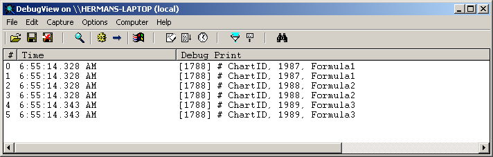
While the procedure may vary for different data providers, quotes that are received in real time will lag in time. Since bar periods during live data collection are based on your computer clock, quotes may end up in the next bar due to their delayed arrival. The data used to backfill your database come from a different data server and will be time stamped. This allows AmiBroker to correct the position of quotes that were received out of sequence. This process removes the real time delays that were present when the data was received.

Since there are no delays with backfilled data, your backfilled data look ahead by several hundred milliseconds with respect to the data you will eventually be trading.

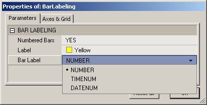
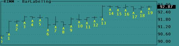
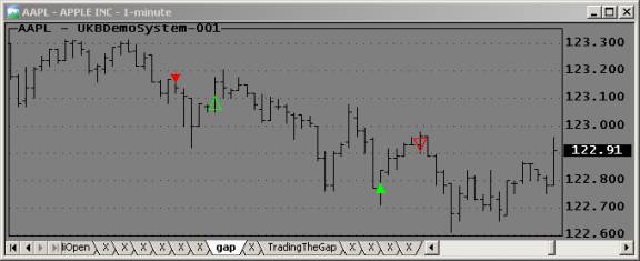
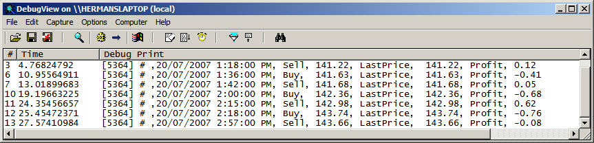
It is not unusual to develop a system with 5-second backfilled data (where all bad ticks and time-stamp errors have been corrected by the data provider) and obtain Holy Grail performance only to find out that when traded with real-time streaming data (where the data is delayed, contains bad ticks and time-stamp errors), the system is a total failure. The following charts illustrate this problem. The data to the left of the red line is backfilled and the data to the right of the Red line is data collected in real time. White is the equity.

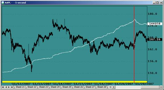
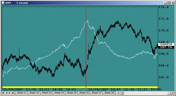
You will not be able to visually judge whether data are backfilled or raw. The differences will only show up by running a trading system on the data; your trading system may be the only way to distinguish between backfilled and raw data. The chart below shows a close up of the data change.

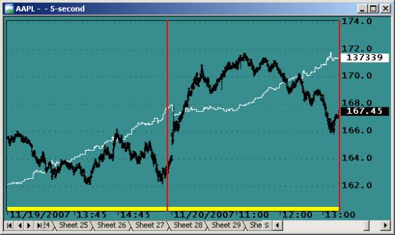
Backfilling the above database and performing another Backtest over the same period produces a very different equity:

There is no guarantee that a system developed on one type of data will perform equally well with the other. When you first encounter a major equity drawdown, you may assume that this was just “a bad day”; after all, all trading systems have them. You may have developed and backtested your system over thousands of trades, covering a period of six months or more. You have been a good student and have used all the recommended methods to validate your trading system. You have tested in- and out-of-sample, applied intelligent optimizations, used Walk-Forward testing, performed Monte-Carlo analysis, and the list goes on. After being so thorough, how could you go wrong? You are ready to trade real money tomorrow and make your first 50% in one day!

The point is that all this effort is wasted time if the data used during development aren’t 100% identical to what you will be trading with.

The best way to develop an HFAT system is to use real live market data. The earlier you change from local or edemo data to real data, the more time you will save, and the more disappointments you will be spared. An HFAT system can never be completed off line, with a local database, or with simulated edemo Data. Its design must always include a significant paper trading and real-money phase.

Another problem when trading your IB paper-trading (simulated) account is that the user does not know the rules Interactive Brokers uses to decide whether an order should be executed or not. These execution criteria may change without warning. This imposes an artificial order to your executions that is unreal; the simulated market conditions will be different from those encountered in real trading. You may well develop a trading system that exploits IB’s way of processing to give you unreal performance, but such a system would fail in real trading.

Also, your paper-trades are not seen by, and cannot influence, the market. When trading real money your orders could be setting a new High or a Low, or if you are trading large sums, you could draw the price up or down. This means that even if your system performs extremely well in simulated trading, this is no guarantee that your system will perform well trading real money.

Using your simulated account to validate your system should never be your final validation before trading for profits; you should always include a real-money evaluation phase in your development plan. Your first real trades should never be to make money; they should be planned to validate your system under varied conditions.

Market behavior is very complex; be prepared for the unexpected and never skip a development step because something works extremely well. For example you might be testing your system using your IB simulated paper-trading account and see your profits skyrocket too fast to follow, perhaps having 90% winners and RARs that are out of this world. When this happens, it is extremely exciting and fun to watch; it is a rare experience that must be appreciated. It suggests that Holy-Grails are possible. But are they? Such favorable trading conditions may last for a few hundred trades, a few hours, or perhaps a few days. This can happen when technical conditions and market behavior are all just perfect for your system. Some unknown factor just made everything work perfectly. When you experience this, you’ll be analyzing your charts, trading log, execution report, etc. for weeks to follow. The fact is that it may never happen again, and you may never know what really happened.

Order and Position Status

IB Position size reporting may be erratic, is always delayed, and may include transient information. If you are trading fast and you use the IB Position Size to determine your next action, this will be a problem. This is especially the case with reversal systems where Covers may be processed before the Buys, and there may be many partial fills. For example, if you are reversing 100 shares, going alternatively Long and Short, you might read position sizes of 0, 100, 200, and even 300 shares. Do not base your system’s action solely on a single reading of the position size; your protective mechanisms will shut down your system many times a day. If a position is not what it is supposed to be on 5 consecutive queries (at quote interval), you may want to close all positions, suspend operation and continue later, or shut down the system and retry later.

Reporting of order status appears more reliable and stable. Usually it seems unnecessary to repeat Order Status queries.

IB Snapshots

Not addressed in this post is the matter of Snapshots however it is extremely important for real-time traders to understand how IB compresses and transmits its data. This topic has been discussed on several forums, for more information on IB data in general please read the following threads:

AmiBroker user group: Interactive Brokers Plug-in dropping volume data
IB’s Discussion Board: Globex Ticks snapshot or reality?
AmiBroker User Group: AB Tick Bar Analysis

The IB Maximum Message Rate

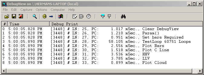
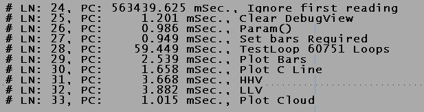
IB has a limit to the maximum rate of messages (order related) you can transmit per second. The rate of queries is not limited. The current limit is 50 messages per second. If you exceed this rate, IB will produce an error code, and if you continue to exceed the message rate, IB will suspend your connection. This, of course, should be prevented at all cost. The message rates are documented here. How to introduce real-time delays measuring in milliseconds is documented in the post on High Precision Interval and Delay Timing.

Internet Delays

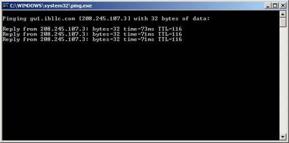
Order and Position status is subject to a 50-400 milliseconds Internet delay. This delay will vary with your location and type of Internet connection to IB. You can test this delay by pinging the IB server. To do this type ping gw1.ibllc.com on command in the Start->Run windows (for Windows XP), and click the run button. A window, as shown below, will appear and show you the delays for three consecutive queries (pings) to IB:

If you encounter excessive delays or cannot connect at all, you can get more details about how your connection is routed by running tracert gw1.ibllc.com in the same manner. You may want to browse the Technical FAQ at IB for related items.

Edited by Al Venosa.

Filed by Herman at 8:55 am under Real-Time System Design
Comments Off on High-Frequency Automated Trading (HFAT); Part 1

Before continuing with this post you should carefully read the AmiBroker Help topic for the getPerformanceCounter().

Measuring time is an important aspect of all real-time intraday trading systems. Typical tasks requiring high-resolution timing include:

1. Limiting the message rate to Interactive Brokers (IB) to 50/sec (API Error 100).
2. Inserting small delays before polling IB Status, to allow for Internet delays.
3. Staggering (interlacing) portfolio trades to spread out the action.
4. Measuring and optimizing AFL execution time.
5. Modifying orders after a small delay (to ensure fills).
6. Periodic execution of tasks, for example, Watchlist scanning, Display and Status refresh, calculations based on slow changing variables, etc.
7. Time-Stamping events, for example order placement.
8. Collecting/preprocessing quotes.
9. Overlay live tick-charts on faster and easier to manage 1-minute charts.

Most of these tasks can be accomplished using just three custom timing functions:

1. GetElapsedTime(): A function that returns elapsed time since reset.
2. SetDelay(): A function that returns time left to reach a future time.
3. GetDelayTrigger(): A function that returns a trigger when a delay times out.

This post provides example functions in a demo application. To allow the use of many timers each function requires you to provide a TimerName, which will be used to retrieve timer information. Static variables are Global and can be read from anywhere; this means you have to be careful not to cross-reference the timers by using the same TimerName from different panes or windows. When running multiple copies of the same code you will need to key the TimerNames. For more on how to do this, see Keying Static Variables in the Real-Time AFL Programming category.

The timers below are implemented using the getPerformanceCounter(). This function returns the amount of time elapsed since the computer was last started. Tomasz recently explained this as follows: “The underlying high frequency counter runs all the time since computer start. What ‘reset’ flag really does is to store last value so next time you read it, it gets subtracted from last value giving you the difference. If reset is false, the last value is set to zero, and you get the original number of ‘clock ticks’ since computer start“.

The timers in this post do their own sampling of the underlying high frequency counter, and the getPerformanceCounter() Reset argument is always left set to False.

The getPerformanceCounter() returns values with microsecond resolution; however, the practical accuracy is severely limited by interruptions from the computer’s operating system. Do not expect much better than about 50-millisecond absolute accuracy. Aside from designing your own dedicated trading hardware (to replace the PC) there isn’t much that can be done about this. If you are brave, you can experiment with increasing program priority in your Task Manager window.

Chart refreshes are most often initiated by an arriving quote, but they can also be initiated by mouse clicks, tooltip, and various chart operations. This means that, when market activity is low and things are not happening as fast as you would like, you can force extra AFL executions by clicking on your chart. You can verify this by running the code below and, while clicking rapidly on the chart, observe that the timer counts displayed will update more rapidly.

You can ensure a one-second chart refresh by adding a RequestTimedRefresh(1) to your code. If the frequency of your arriving data is slow, your AFL code may execute only sporadically. Since your code must execute to read your timers, the resolution of your timers will be limited by the chart refresh rate. If your chart refreshes once a second your timing resolution will be one second!

Normally most of the AFL code in an Indicator window executes when your chart refreshes; however, to obtain speed advantages, you may execute non-critical sections (like account information and System Status) of your code less frequently using a timer. You can also execute small sections of code more frequently by placing them inside a well-controlled loop. If you do this, be sure to limit the maximum time your code can spend inside the loop to one second or less.

For fast trading systems, the frequency of AFL executions (chart refreshes) may be slow and this may make it difficult for you to get LMT fills. There is no way to have a program that requires 50 milliseconds per pass to execute 20 times per second.

Considering the interval between AFL executions, it is important to plan the layout of your code so that all events are handled in the most efficient order. If you don’t, transmittance of your order could well be delayed by up to a full second. There are situations where you want to invoke an immediate re-execution of your code. In some cases you might want to do this after placing an order to check order status before the next quote or refresh. Although it should be used sparingly this is possible by calling the RefreshAll():

<p>This function can only be called once a second; calling it faster will not result in more frequent chart refreshes. This means you should only call it when really needed. <p>The code presented below is for demonstration only. The getElapsedTime() lets you measure elapsed time from the moment of Reset. The first argument passes the name you assign to the static timer; this allows you to use the same function to time different events. The second argument is a Reset flag. When this Reset is True, the function samples the underlying high frequency counter and uses it for later reference. When you call the function with the Reset argument set to False, it calculates the elapsed time by subtracting the earlier sampled value from the current value of the Performance Counter. <p>The setDelay() function lets you Start, Read, and Cancel a time delay. The TimerName argument functions as in the getElapsedTime(). Calling the setDelay() with the mSecDelay argument set to a non-zero value will start the Delay timer. Calling it with the mSecDelay argument set to zero will make it return the current count-down time in millseconds. Calling the function with the cancel argument set to True will terminate the delay. <p>The getDelayTrigger() function returns a trigger. This is a signal that is true for only one pass through the code. Triggers are frequently used in real-time trading systems. They are needed to prevent multiple actions when a signal becomes True. <p>To run the code, copy the formula to an Indicator and click Insert. You'll see a chart window like Figure 1 below: 

<p align="center">Figure 1. Result from running the example code. 
<a href='http://www.amibroker.org/userkb/2007/11/10/high-precision-delay-and-interval-timing/timerdisplayjpg/' rel='attachment wp-att-1422' title='timerdisplay.jpg'><img src='http://www.amibroker.org/userkb/wp-content/uploads/2007/11/timerdisplay.jpg' alt='timerdisplay.jpg' /></a>

<p>The example code maintains three timers, T1, T2 and T3. All timing values are expressed in milliseconds. In Figure-1 the Elapsed Time shown is measured from timer Reset. The Delay shown is the time remaining after Start, until the delay times out. The line for Timer T2 shows that its Delay just timed-out and produced a trigger. Timer T3 still has a Delay in progress. Right-click on the chart to open the Param window: 

<p align="center">Figure 2. Param window. 
<a href='http://www.amibroker.org/userkb/2007/11/10/high-precision-delay-and-interval-timing/timerparampng/' rel='attachment wp-att-1423' title='timerparam.png'><img src='http://www.amibroker.org/userkb/wp-content/uploads/2007/11/timerparam.png' alt='timerparam.png' /></a>

<p>If you click one of the timer Resets in the Param window you'll see the ElapsedTime in the corresponding row go to zero, and then start to increment sporadically when your chart refreshes. Without live data this would be at approximately 1-second intervals, as determined by the RequestTimedRefresh(1); <p>If you click Start for one of the timers this will start a delay. You can see how it counts down in the Delay column. Click the timer's Cancel to terminate the Delay. Note that whenever a Delay times out, the word "Trigger" briefly appears in the third column. 


function RefreshAll()
    {
    oAB = CreateObject("Broker.Application");
    oAB.RefreshAll();
    }

function getElapsedTime( TimerName, Reset )
    {
    if( Reset ) 
        {
        TimeRef= GetPerformanceCounter(False);
        StaticVarSet(TimerName,TimeRef);
        }
    TimeRef = Nz(StaticVarGet(TimerName));
    ElapsedTime = GetPerformanceCounter(False) - TimeRef;
    return ElapsedTime;
    }

function setDelay( TimerName, MsecDelay, Cancel )
    {
    HRCounter= GetPerformanceCounter(False);
    if( Cancel ) 
        {
        StaticVarSet("TO"+TimerName,-1);
        StaticVarSet("DS"+TimerName, 0);
        }
    else if( MsecDelay ) 
        {
        StaticVarSet("TO"+TimerName,HRCounter+MsecDelay );
        }
    TimeOutTime = Nz(StaticVarGet("TO"+TimerName));
    DelayCount = Max(0, TimeOutTime - HRCounter );
    StaticVarSet("DC"+Timername, DelayCount);
    return DelayCount;
    }

function getDelayTrigger( TimerName )
    {
    DelayCount = Nz(StaticVarGet("DC"+TimerName));
    DelayState = DelayCount > 0;
    PrevDelayState = Nz(StaticVarGet("DS"+TimerName));
    StaticVarSet("DS"+TimerName, DelayState);
    return DelayState < PrevDelayState;
    }
 
RequestTimedRefresh( 1);

_SECTION_BEGIN("TIMER 1");
Reset1 = ParamTrigger("1 - Reset","RESET");
MSecDelay1 = Param("1 - Delay (mS)",1000,0,10000,10);
if( ParamTrigger("1 - Start", "START") ) setDelay( "Timer1", MSecDelay1, 0 );
if( ParamTrigger("1 - Cancel", "CANCEL") ) setDelay( "Timer1", MSecDelay1, 1 );
_SECTION_END();

_SECTION_BEGIN("TIMER 2");
Reset2 = ParamTrigger("2 - Reset","RESET");
MSecDelay2 = Param("2 - Delay (mS)",4000,0,10000,10);
if( ParamTrigger("2 - Start", "START") ) setDelay( "Timer2", MSecDelay2, 0 );
if( ParamTrigger("2 - Cancel", "CANCEL") ) setDelay( "Timer2", MSecDelay2, 1 );
_SECTION_END();

_SECTION_BEGIN("TIMER 3");
Reset3 = ParamTrigger("3 - Reset","RESET");
MSecDelay3 = Param("3 - Delay (mS)",8000,0,10000,10);
if( ParamTrigger("3 - Start", "START") ) setDelay( "Timer3", MSecDelay3, 0 );
if( ParamTrigger("3 - Cancel", "CANCEL") ) setDelay( "Timer3", MSecDelay3, 1 );
_SECTION_END();

ET1     = getElapsedTime( "Timer1", Reset1 );
ETA1     = setDelay( "Timer1", 0, 0 );
TT1     = getDelayTrigger( "Timer1");

ET2     = getElapsedTime( "Timer2", Reset2 );
ETA2     = setDelay( "Timer2", 0, 0 );
TT2     = getDelayTrigger( "Timer2");

ET3     = getElapsedTime( "Timer3", Reset3 );
ETA3     = setDelay( "Timer3", 0, 0 );
TT3     = getDelayTrigger( "Timer3");

Title = "\nFilename: "+Filename+"\n\n"+
"MilliSeconds Since Computer Startup: "+NumToStr(GetPerformanceCounter(False),1.3)+"\n\n"+
"Timer     ElapsedTime     Delay     Trigger\n\n"+
"T1      "+NumToStr(ET1,10.0)+"     "+NumToStr(ETA1,7.0)+"      "+WriteIf(TT1,"TRIGGER1","")+"\n\n"+
"T2      "+NumToStr(ET2,10.0)+"     "+NumToStr(ETA2,7.0)+"      "+WriteIf(TT2,"TRIGGER2","")+"\n\n"+

Edited by Al Venosa.

Filed by Herman at 9:09 pm under Real-Time AFL Programming
Comments Off on High-Precision Delay and Interval Timing

Backfilling data can be done in many ways, and different methods may be needed for different data providers. The method shown below was developed for eSignal data. If you use another data provider, you may need to modify the code and the procedure.

When backfilling data, you should confirm that data are backfilled properly and have some indication regarding the presence of data holes. As pointed out in Data Holes in Real-Time Trading, to be able to detect holes, you need a perfect data array against which to compare the data. Since AmiBroker doesn’t have such a data array, the method presented here uses the QQQQ as a reference ticker. Turn ON and set Backtester Settings -> General -> Pad and align all data to reference symbol -> QQQQ. To have all tickers backfilled, you should also turn ON Wait for Backfill(RT only). To speed up real-time backfills you may want to display only a simple price chart, instead of complex code. Refreshing complex Indicators or Systems will slow down backfill. The following Exploration will Backfill all tickers in your Watchlist and report on it’s success:

Filed by Herman at 11:56 pm under Real-Time AFL Programming
Comments Off on Backfill Exploration for Real-Time data

In real-time trading it is vital to keep your chart right justified, i.e., ensuring the right-most price bar is visible at all times. Failing to do so and looking at the wrong bar when trading real-money can invoke a panic response by the trader that results in erroneously closing a position or worse, placing a wrong order. This can easily happen if you are running several computers and are not always monitoring the chart being traded.

The following code shows you how you can right-justify your chart at system startup or from the Param window. A visible alert that changes the chart back ground color when the last bar is not visible is included.

The Alarm uses DateTime() to automatically correct for blank bars at the right edge of your chart. The code is kept explicit and you may be able to optimize it for speed.

<p>

Edited by Al Venosa.

Filed by Herman at 12:41 pm under Real-Time AFL Programming
Comments Off on Keeping Your Chart Right-Justified

When you are developing systems and discussing charts with other traders by email, it is often convenient to be able to refer to the bars on your chart by number, date, or time. The code below can be appended to the end of your code to give you these options:

The b < Barcount check prevents out of range errors when you have AmiBroker Preferences set to give you a number of Blank bars at the right edge of your chart.

Plot(C,"",1,128); 
_SECTION_BEGIN("BAR LABELING"); 
ShowBars = ParamToggle("Label Bars","NO|YES",0);
LabelCo = ParamColor("Label",colorYellow);
Label = ParamList("Bar Label","NUMBER|TIMENUM|DATENUM",0); 
GraphXSpace = 10; 
if( Showbars ) 
{ 
DN=DateNum(); 
TN=TimeNum(); 
FirstVisibleBar = Status( "FirstVisibleBar" ); 
Lastvisiblebar = Status("LastVisibleBar");  
for( b = Firstvisiblebar, BN=0; b <= Lastvisiblebar AND b < BarCount; b++) 
{ 
if( Label == "NUMBER" ) BarLabel = NumToStr(BN++,1.0); 
else if ( Label == "TIMENUM" ) BarLabel = NumToStr(TN[b],1.0); 
else BarLabel= NumToStr(DN[b],1.0); 
PlotText("\n^\n"+BarLabel,b,L[b],LabelCo); 
} 
} 
_SECTION_END();

The labeled charts look like this:

Below a more streamlined version using the Switch():

_SECTION_BEGIN( "BAR LABELING" );
Plot( C, "", 1, 128 );
ShowBars = ParamToggle( "Label Bars", "NO|YES", 0 );
LabelCo = ParamColor( "Label", colorYellow );
Label = ParamList( "BarLabel", "NUMBER|TimeNum|DateNum|BARNUM|WEEKDAYNUM|WEEKDAY", 0 );
GraphXSpace = 10;

if ( Showbars )
{
    DN = DateNum();
    TN = TimeNum();
    WD = DayOfWeek();
    WDList = "SUN,MON,TUE,WED,THU,FRI,SAT";
    FirstVisibleBar = Status( "FirstVisibleBar" );
    Lastvisiblebar = Status( "LastVisibleBar" );

    for ( b = Firstvisiblebar, BN = 0; b <= Lastvisiblebar AND b < BarCount; b++ )
    {
        switch ( Label )
        {
            case "NUMBER":
                BarLabel = NumToStr( BN++, 1.0 );
                break;
            case "TIMENUM":
                BarLabel = NumToStr( TN[b], 1.0 );
                break;
            case "BARNUM":
                BarLabel = NumToStr( b, 1.0 );
                break;
            case "WEEKDAYNUM":
                BarLabel = NumToStr( WD[b], 1.0 );
                break;
            case "WEEKDAY":
                BarLabel = StrExtract( WDList, WD[b] );
                break;
            default:
                BarLabel = NumToStr( DN[b], 1.0 );
                break;
        }
        PlotText( "\n^\n" + BarLabel, b, L[b] - ( H[b] - L[b] ), LabelCo );
    }
}
_SECTION_END();

Edited by Al Venosa.

Filed by Herman at 4:10 pm under Debugging AFL
Comments Off on Numbering Bars

When your code increases in complexity, it will start to execute more slowly, and you will eventually reach a point where you will want to optimize your code for speed of execution. Even if you are willing to buy a faster computer, it will rarely give you a greater speed advantage than optimizing your code.

Important note: The AmiBroker 5.01.1 beta released on 5/10/2007 offers a new profiling function that enables you to get accurate performance timing for all AmiBroker and custom functions called. It is available from the AFL Editor: Tools -> Code Check and Profile menu. To use this new tool effectively you should convert your code modules to function calls as much as possible. Try it!

The first requirement for analyzing your AFL execution speed is the ability to measure the execution times. This is best done using the GetPerformanceCounter(), which gives microsecond resolution. You can display the execution time in the chart Title, or log them to DebugView. To get an appreciation of how fast AFL executes you may want to time a few of your most frequently used AFL statements. As Tomasz pointed out in his comment to an earlier version of this post, this can be done using a simple loop:

<p>On my 2GHz laptop, the Param() takes about 4 microseconds to execute. The "Statement under test" can be any AFL statement or section of code you want to analyze. This simple code will give you a fairly accurate idea of the true execution time. Please do not forget that all&nbsp;programs executing under Microsoft Operating Systems&nbsp;are subject to interruptions. This means that your readings may fluctuate and will generally be greater than their absolute true values. Your normal program executions are&nbsp;also subject to these interruptions and, if you perform&nbsp;precision timing tasks, your should consider their effect.</p> 

<p>If, in view of processing overhead, you prefer not to use DebugView, you can log execution times either to the Interpretation screen, which invokes an additional AFL execution, or to the chart Title if you output just a few measurements. Use of DebugView is outlined in several posts in the <a href="http://www.amibroker.org/userkb/category/real-time-auto-trading/debugging-afl/">Debugging AFL</a> category. When you are logging to DebugView, execution times will be inflated by the amount of time needed to call and execute the _Trace() functions. You can measure the timing overhead for a single&nbsp;_Trace()&nbsp;function using the same method we used above:</p> 


<p>On my 2GHz laptop, the _Trace() takes about 35 microseconds to execute. Compared to the Param(), this would appear like a major error, but in practice it is not. For example, when calling the&nbsp;_Trace() function thirty times in your code, this would add only about 1 millisecond to the overall execution time of your program. </p> 

<p>The example code below logs to DebugView and to the chart Title. It uses a small Trace() function that is called each time you want to log a timing measurement. You can customize this function to log additional information. Although you can call this function on each line, you do not have to. Calling Trace() introduces a small measurement error. This means that when you remove the measurement code, performance should be slightly better than your measurements predict. If you do not use DebugView, you can delete all DebugView related statements. If you do this, I suggest you comment them out until your modified code has been verified.</p> 

<p>Be careful when calling the Trace() from inside a loop. If your loop steps through 50,000 bars of data, inserting one or more Trace() calls will slow down your code substantially and result in a significant measurement error. The key to reasonable accuracy is to use the minimum number of _Trace() statements and keep them out of loops and frequently called functions.</p> 

<p>Inserting/removing TRACE() statements in a test program is easily done using the Edit- Replace function in the formula editor. To add _Trace() statements, replace the ";" at the end of the line with "; TRACE("");":</p> <p align="center"><img height="178" src="http://www.amibroker.org/userkb/wp-content/uploads/2007/09/clip-image0023.jpg" width="351" border="0"></p> 

<p>To remove the _Trace() statements substitute "; TRACE("");" with ";":</p> <p align="center"><img height="178" src="http://www.amibroker.org/userkb/wp-content/uploads/2007/09/clip-image0043.jpg" width="351" border="0"></p> 

<p>Place your cursor just before the last ";" that precedes the first line of code you want to time. Stop substitutions where you no longer want to time statements. You should initialize the LineNumber to the line number that contains your first Trace() statement. Line numbers for your cursor position are displayed at the right bottom of your editor screen.</p> 

<p>Here is a do-nothing program where _Trace() statements were added using the above method. You can modify the function Trace() to output any information you like: 

<p>function Trace( Comment )</p> <p>{</p> <p>global LineNumber, TitleStr;</p> <p>PC = GetPerformanceCounter( True );</p> <p>Str = "# LN: "+NumToStr(LineNumber++,1.0,False)+", PC: "+NumToStr(PC,9.3)+" mSec., "+Comment;</p> <p>TitleStr = TitleStr + Str+"\n";</p> <p>_TRACE(Str);</p> <p>}</p> 
<p>

The output produced in DebugView looks like this:

The output in the Title looks like this:

The first reading in the Title should be ignored as it initializes the PerformanceCounter. This reading is suppressed by the DBViewClear command in the DebugView log. The above method can be used to determine execution times of all AFL functions. Note that in the above example SetBarsRequired() is used to process all available data. This would be the worst-case measurement. Commenting out SetBarsRequired() will make your code execute under Quick-AFL. This may be significantly faster than running over all data.

Measuring Execution Order and Timing for Window Panes

When you are executing AFL formulas in multiple panes or windows and experience a timing problem, the first step to take, before using the above method, is to determine which pane uses up too much time. You can turn on Tools -> Preferences ->Miscelaneous -> Display Chart Timing to read the execution time at the bottom of the charts. Alternatively, the simple code below lets you log the execution order and time for the formulas in each open pane to DebugView. Since the AmiBroker Performance Counter readout is unique for each pane, the code below does not use it. In this case you will have to turn on Options -> Show Milliseconds in DebugView. This will give you Millisecond resolution, not micro-second as with the performance Counter and is a very approximate measurement. It should only be used to identify the problem formula. The execution order of the panes is revealed by the order in which the lines appear in the DebugView.

Filename = StrLeft(_DEFAULT_NAME(),StrLen(_DEFAULT_NAME())-2);
function TraceChartID() 
{ 
Msg = "# ChartID, "+NumToStr(GetChartID(),1.0,False)+", "+Filename;
_TRACE( Msg ); 
return Msg;
} 

TraceChartID();

//
for(n=0; n<BarCount;n++) ; // your code would be here
//

Title = TraceChartID(); 

The Filename assignment and the TraceChartID() should be placed at the very top of your code, or you can add it to your default Include file. The single line used to call this function should be placed at both the beginning and the end of the code in each window/pane. This is what it looks like in DebugView:

Edited by Al Venosa.

Filed by Herman at 3:44 pm under Real-Time AFL Programming
Comments Off on Measuring AFL Execution Times (v3)

This post shows how to add intraday session timing to the Real-Time Gap-Trading (RTGT) system developed in the previous post. However, before tackling session timing, there are a few things you should be aware about:

Time-Synchronization

In real-time trading there are many functions that are timed with reference to your system’s clock. It is therefore imperative that you always synchronize your computer clock with an Internet timeserver before each trading session.

Tools -> Preferences -> Intraday settings

Data Timestamps can be aligned to either the start or the end of the base period. The code developed here uses time of FIRST tick inside bar, i.e., the data timestamp returns the time at the start of the bar. This is when the first quote for the new period arrives and defines the Open for the new bar. Click Tools -> Preferences -> Intraday to set this option:

Backtesting and Bar-Replay

During backtesting the timing resolution will be equal to the periodicity set in AA Settings. If you are comparing Backtester signals with the signals displayed on your chart, you must make sure that the AA and Chart use the same periodicity.

During Bar Replay the timing resolution will be equal to the greater of the base interval of your database or the Step Interval selected in the Bar-Replay window.

During Backtesting and Bar-Replay, AmiBroker will refer to the timestamp to know how prices change over time. Hence, you will have no choice but to time events, such as session timing, with reference to the data timestamp.

Live Trading

When trading from an Indicator, the data timestamp is rounded to the selected chart-periodicity, i.e., if you display a 1-minute chart, the timing resolution will be one minute. This means you cannot implement delays based in seconds using the data timestamps of a minute database. This is why most functions in a real-time trading system use the computer clock as reference.

You can, with caution, use either the data timestamp or the system’s clock to control your session. However, since the data timestamp is dependent on the arrival of new quotes (ignoring data padding), using data timestamp could be unreliable. If you want higher timing resolution, you could create a 5-second database. However, this means working with slow backfills and slow AFL executions, due to lengthy data histories. To keep things simple, we will use a one-minute database.

Session Timing

When you are developing real-time trading systems, it is often handy, even essential sometimes, to develop several code versions. Typically, these might include:

1) A version for Backtesting and Bar-Reply. This version would use the TimeNum function for timing.
2) A Real-Time trading version. This version would use the system clock (Now()) for timing and would be highly optimized for AFL execution speed.
3) A DebugView version. This is a useful intermediate development stage that lets you run your system in real-time without any TWS interfacing; it logs trades to DebugView instead of sending them to the TWS.

ParamTime() input statements are used to set the start- and end-time of the trading session. The code below is only intended for preliminary system evaluation using the Backtester: hence, is uses time-numbers for session timing.

The StartOfSession and EndOfSession variables are triggers (they last only one bar). They are used to initialize processes at the start of the session and clean up processes at the end of the session. The InSessionTime variable is True during trading and is used to control processes that must be turned On/Off depending on whether you are trading or not. These processes will be covered in future posts.

A TimeFrame Parameter has been added to help visualize how the system works in different timeframes. To see the equity for different timeframes, just drag the slider to see the system response to any timeframe from 1 minute to 1 hour. Having added Session Timing you can now explore whether this system is more profitable during certain hours of the trading day. I suggest you perform an individual backtest on you favorite watchlist; you may be surprised to find that with some systems there is no need to trade all day. More…

For debugging purposes, you can turn On/Off a colored ribbon to display the Start- (Green), End- (Red) and In-Session (Yellow) variables.

For convenience the code below includes all previously developed parts. Just copy to an Indicator formula window, and click Apply.

<p>_SECTION_BEGIN("SESSION TIMING"); 
<p>TimeFrame= Param("Chart Timeframe (min)",1,1,60,1)*60; <p>TimeFrameSet(TimeFrame); <p>TN = TimeNum(); <p>ParamStartTime = ParamTime("Session Start","09:30:00"); <p>ParamEndTime = ParamTime("Session End","15:59:00"); <p>InSessionTime = TN &gt;= ParamStartTime AND TN &lt;= ParamEndTime; <p>StartOfSession = InSessionTime &gt; Ref(InSessionTime,-1); <p>EndOfSession = InSessionTime &lt; Ref(InSessionTime,-1); <p>InsessionTime = InSessionTime OR EndOfSession;
<p>_SECTION_END();

<p>Buy = O &lt; Ref(L,-1) AND InsessionTime; <p>BuyPrice = O; <p>Sell = L &lt; Ref(L,-1) OR EndOfSession; <p>SellPrice = C; <p>Short = O &gt; Ref(H,-1) AND InsessionTime; <p>ShortPrice = O; <p>Cover = H &gt; Ref(H,-1) OR EndOfSession; <p>CoverPrice = C; <p>SetTradeDelays(0,0,0,0); <p>SetOption("CommissionMode",3); <p>SetOption("CommissionAmount", 0.005); <p>E=Equity(1); <p>TradeEquity = ValueWhen(Sell OR Cover,E); 

<p>_SECTION_BEGIN("PLOTTING");
<p>Plot(C,"",1,128); <p>if( ParamToggle("Session Timing Ribbons","HIDE|SHOW",0) ) <p>{ <p>Plot( InSessionTime,"",7,styleArea|styleOwnScale|styleNoLabel,0,60); <p>Plot( StartOfSession,"",5,styleArea|styleOwnScale|styleNoLabel,0,30); <p>Plot( EndOfSession,"",4,styleArea|styleOwnScale|styleNoLabel,0,30); <p>} <p>OutOfSessionColor = ParamColor("Out of Session",colorDarkRed); <p>Plot(NOT InSessionTime,"",OutOfSessionColor,styleArea|styleOwnScale|styleNoLabel,0,1); <p>PlotShapes(IIf(Buy, shapeSmallUpTriangle, shapeNone),5,0,BuyPrice,0); <p>PlotShapes(IIf(Sell, shapeHollowDownTriangle, shapeNone),4,0,SellPrice,0); <p>PlotShapes(IIf(Cover, shapeHollowUpTriangle, shapeNone),5,0,CoverPrice,0); <p>PlotShapes(IIf(Short, shapeSmallDownTriangle, shapeNone),4,0,ShortPrice,0); <p>if(ParamToggle("Equity curve","HIDE|SHOW",0) ) <p>{ <p>Plot(TradeEquity,"",2,styleStaircase|styleOwnScale); <p>}

Filed by Herman at 2:07 pm under Real-Time System Design
Comments Off on Gap-Trading demo, Session Timing Example

This system was intended to provide signals to demo trade automation. However, its signals are not that frequent and it proved to be quite boring to automate it. The code is left here but I plan to use another system to demo trade automation. You may also note that I separated Real-Time System Design from System Automation. This was done to allow categories to evolve independent from each other.

To develop trade-automation code we need a demo system to generate signals and to test TWS interfacing. To be able to continue this series and not waste time looking for a superb system, I’ll use the following very simple trading rules:

Buy at the Open of the current bar if it falls below the previous Low.
Sell at the Close when the current Low falls below the previous Low.
Short at the Open when the Open exceeds the previous High.
Cover at the Close when the current High exceeds the previous High.

In AFL this looks like this:

SetOption("CommissionMode",3);
SetOption("CommissionAmount", 0.005);
SetTradeDelays(0,0,0,0);
Buy = O < Ref(L,-1);
BuyPrice = O;<br>Sell = L &lt; Ref(L,-1);
SellPrice = C;<br>Short = O &gt; Ref(H,-1);
ShortPrice = O;<br>Cover = H &gt; Ref(H,-1);
CoverPrice = C;
E=Equity(1);<br>Plot(C,"",1,128);
if( PlotTriangles = ParamToggle("Triangles","HIDE|SHOW",1) )
{
PlotShapes(IIf(Buy, shapeSmallUpTriangle, shapeNone),5,0,BuyPrice,0);
PlotShapes(IIf(Sell, shapeHollowDownTriangle, shapeNone),4,0,SellPrice,0);
PlotShapes(IIf(Cover, shapeHollowUpTriangle, shapeNone),5,0,CoverPrice,0);
PlotShapes(IIf(Short, shapeSmallDownTriangle, shapeNone),4,0,ShortPrice,0);
}

The above code is a variation of The Full Gap-Trading system. You can read more about this type of system on the Stockcharts site and many other Internet sites.

This system will produce trades in all timeframes, trade frequently, and trade both long and short. Running this system in the 1-15 minute timeframe will give us lots of action and make it easier to develop and debug the Trade-Automation (TA) code. An AT trading system designed around a system that gives only a few signals a day will take forever to debug. Mechanical performance is the first objective.

For now we assume that we can enter at the bar’s Open price. Note that I exit at the Close of the bar because, in the AmiBroker database, this is the next price that is available. At this stage this system is designed to stimulate trade-automation code and not to make you rich; DO NOT TRADE IT. Order types and/or strategies will be decided on later. Trade-Delays are set to zero because they are better handled in the code. The Equity(1) statement is used to remove redundant signals. The indicator should display trades as follows:

Edited by Al Venosa.

Filed by Herman at 5:00 pm under Real-Time System Design
Comments Off on Real-Time Gap-Trading Demo, Basics (v3)

The phenomenon that is the basis of many trading systems is the observation and trading of an exceptional price movement followed by a pullback.

An extreme example of the pullback phenomenon would be a Spike as shown in the chart below. Because the price change is so extreme, the pullback or correction appears instantaneous. There is no clear market response, i.e., traders at large are not inclined to take the price change seriously.

The problem is that inadvertently you can easily write code that trades these spikes. Only when you start trading such a system will you discover that your orders are not filled because the volume just isn’t there. This is a common reason why backtested and real results may sometimes differ substantially. You may have designed a system that is completely rational, backtests perfectly, and stands up to the most detailed technical scrutiny, only to find out that in real trading it fails completely.

You might think that by increasing the timeframe, for example to 15-minute or even daily, you can minimize this problem. However, while doing this may make the spikes less prominent, the tradability will not improve. Consider the spike in the 15-minute chart below:

Adding a few percent bands makes this look like a real trading opportunity. It looks so easy! However, the Low of the bar is still created by a single trade and the chance to get your order filled would still be minimal. Designing trading systems around minimal-volume price changes is one of the easiest traps for a real-time system developer to fall into. When designing an intraday trading system you should design your code to minimize the divergence of the backtester with respect to real-trading results. You can do this by working in the smallest time frame possible. Even when trading at hourly intervals you should write your code in the minute (or even Tick) timeframe.

There are a number of ways in which to do this. Take a look at the 10:30 AM spike in the 15-minute chart below and consider how you would determine its tradability:

The fact is that there is no way to tell whether the 10:30 AM High is tradable. However, expanding the chart to the 1-minute timeframe, as shown below, lets you clearly see a gradual reversal pattern. This means your order could probably have been filled somewhere near the top of the 15-minute spike shown earlier.

Running your Backtester in the 1-minute timeframe and looking for one-bar confirmations may drop your backtester performance, but your results would have been closer to that which can be obtained in real trading. In this case you would have separate Backtester and Trading code versions for your system; the Backtester code would include signal confirmation while your Trading code would not.

Edited by Al Venosa.

Filed by Herman at 6:07 pm under Real-Time System Design
Comments Off on Designing a Tradable System – Spikes

The design of real-time automated trading systems involves two major design phases: 1) Designing the trading system and 2) Developing the trade-automation code. While you may be able to re-use some previously developed AT functions, you can rarely transport the entire automation section from one trading system to the next. Adjusting your AT code to work with a new system can be very time consuming; it can involve weeks of real-time testing and debugging. Using the code below you can test your new system ideas, in a tick environment, before you have written a single line of automation code.

Note that when testing this code with the Bar-Replay tool, the log will display the bar’s closing price instead of the Lastprice (tick data). When testing this code with your own trading system, you may want to add extra output to the _TRACE() statements. The code below substitutes DebugView output for orders that would have normally gone to the TWS:

Filed by Herman at 7:17 pm under Debugging AFL
Comments Off on Order Simulation using DebugView