Users' Knowledge Base

Interactive Brokers’ Real-Time Volume Data

Just like with price data, volume data are subject to delays and BF (Backfill) corrections. Moreover, IB (Interactive Brokers) reports volume data in a manner that could cause major performance differences between backtesting and actual trading.

This post outlines simple procedures to collect RT and BF data for comparison. No effort is made to explain the differences or to perform statistical analysis. The views expressed here are based on personal experiences and/or may be anecdotal; not everything that happens in real-time trading is easy to explain. As always, if you have technical insight and/or see inaccuracies, please comment for the benefit of future readers.

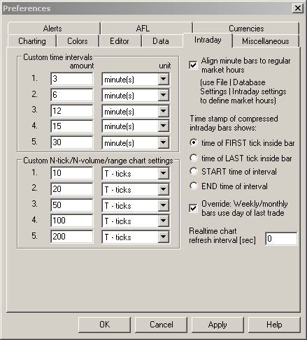
As expected, IB RT volume data contain the usual bad ticks and delays that are corrected during backfill. However, and this is very important to the RT trader, IB adjusts live volumes at about 30-second intervals. This means that the volumes IB reports during RT trading do not accurately reflect market activity. This means also that volume data may be delayed by up to 30 seconds, instead of by the typical snapshot delay, which is about 300 milliseconds for price data. Comparing backfilled with real-time volume, it appears that the real-time periodic volume adjustments are re-distributed across individual snapshots during backfill. This post is intended to help you perform your own data analysis. The methods outlined below are intended to get you started.

To collect and save real-time data:

1. Create a new database in the 5-second interval.
2. Embed “RD”, for Raw Data, when naming the database.
3. In Database Settings select the Interactive Brokers plugin.
4. Pick a high volume stock, for example, AAPL (used in this post).
5. Connect to the TWS (Trader Work Station), signing in to your Paper Trading account. Do not use the eDemo account.
6. Collect about an hour’s worth of real-time data.

The first thing that will happen when you connect to the TWS is that AmiBroker backfills approximately 2000 bars of 5-second data. This cannot be prevented and you must be careful to note the time where backfill ends and raw data collection starts. The simplest way is to place a vertical line on your chart and label it “Start of real-time data”.

To save the database:

1. Disconnect the IB plugin (see Plugin menu at right bottom of chart).
2. Open Database Settings and set the database to Local.
3. Place another vertical line to indicate where data collection stopped.
4. Go to the File menu and save the database.

Be sure to set the Database Settings -> Data Source -> Local before saving. If you do not do this the database will backfill on the next startup and this may corrupt your RT data sample.

The next step is to collect a sample of BF data that overlaps the previously collected real-time sample. To do this, you need to create another database. Since IB backfills only about 2000 bars of 5-second data, you should do this as soon as possible after collecting raw data, else the collection periods may not overlap and you will not be able to compare the two types of data. The procedure is the same as above except that you want to embed “BF” (for backfilled data) instead of “RD” in the database name.

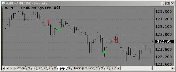
To visually compare the two databases you can open two instances of AmiBroker and load the RT database in one and the BF database in the other. You can then display the two databases at the same time and visually compare the respective charts. You may want to display both a price chart and a volume chart in separate panes, as shown in the captures below.

You can use the code below to inspect your price chart:

<b>Plot</b>(<b>C</b>,<b>"Close"</b>,<b>colorBlack</b>,<b>styleBar</b>); <p>TN=<b>TimeNum</b>(); <p>Cursortime = <b>SelectedValue</b>(TN); <p>CumHL = <b>Cum</b>(<b>IIf</b>(TN&gt;=CursorTime,<b>H</b>-<b>L</b>,<b>0</b>)); <p><b>Plot</b>(CumHL,<b>""</b>,<b>4</b>,<b>styleArea</b>|<b>styleOwnScale</b>); <p><b>Title</b>=<b>Name</b>()+<b>" Interactive Brokers BackFilled price data - "</b>+<b>Interval</b>(<b>2</b>); 

And this code to inspect your Volume chart:

<b>Plot</b>( <b>Volume</b>,<b>""</b>,<b>2</b>,<b>styleOwnScale</b>|<b>styleHistogram</b>|<b>styleThick</b>); <p>TN=<b>TimeNum</b>(); <p>Cursortime = <b>SelectedValue</b>(TN); <p>CV = <b>Cum</b>(<b>IIf</b>(TN&gt;=CursorTime,<b>V</b>,<b>0</b>)); <p><b>Plot</b>(CV,<b>""</b>,<b>4</b>,<b>styleArea</b>); 
<p><b>Title</b>=<b>"Backfilled Volume data - "</b>+<b>Interval</b>(<b>2</b>); 

The above formulas will display basic charts plus a cumulative value (red area) for any parameter you would like to test. In the price chart, high-low range (H-L) is summed while in the Volume chart plain Volume is summed. Summation starts with the cursor-selected bar. This feature is only provided to visually reveal data differences; it has no other significance.

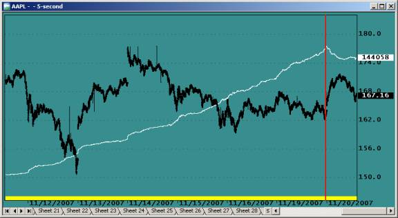
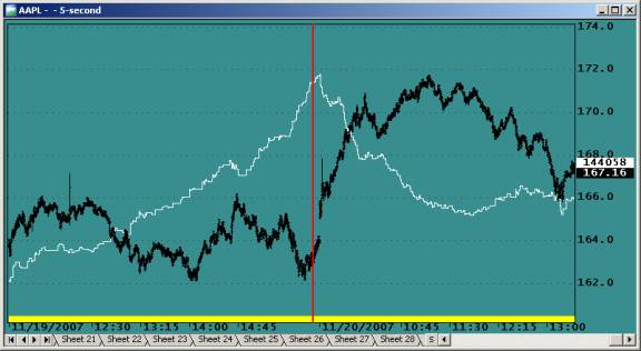
The charts below were created using the above methods, which quickly reveal the difference between the two types of data. To explain why these difference occur is left up to the expert reader (because I don’t have a clue!!).

Figure 1 – Backfilled data

Figure 2 – Real-Time Collected data

The following volume indicator can be used to display the RT volume periodicity more clearly:

Filename = <b>StrLeft</b>(_DEFAULT_NAME(),<b>StrLen</b>(_DEFAULT_NAME())-<b>2</b>); <p>Vref = <b>Ref</b>(<b>HHV</b>(<b>V</b>,<b>4</b>),-<b>1</b>); <p>VSpike = <b>V</b> &gt; Vref <b>AND</b> <b>V</b>&gt;<b>Ref</b>(VRef,-<b>1</b>)/<b>2</b>; <p>BS=<b>ValueWhen</b>(VSpike,<b>BarsSince</b>(<b>Ref</b>(VSpike,-<b>1</b>))+<b>1</b>); <p><b>Plot</b>(<b>V</b>,<b>""</b>,<b>2</b>,<b>styleHistogram</b>); <p><b>Plot</b>(<b>IIf</b>(Vspike ,<b>V</b>,<b>Null</b>),<b>""</b>,<b>1</b>,<b>styleArea</b>); <p>FirstVisibleBar = <b>Status</b>( <b>"FirstVisibleBar"</b> ); <p>Lastvisiblebar = <b>Status</b>(<b>"LastVisibleBar"</b>); <p>TN=<b>DateTime</b>(); <p>S=<b>Second</b>(); <p><b>for</b>( b = Firstvisiblebar; b &lt;= Lastvisiblebar <b>AND</b> b &lt; <b>BarCount</b>; b++) <p>{ <p><b>if</b>(VSpike[b]) <b>PlotText</b>( <p><b>"\n"</b>+<b>NumToStr</b>(<b>V</b>[b]/<b>100</b>*<b>Interval</b>(),<b>1.0</b>,<b>False</b>)+ <p><b>"\n"</b>+<b>NumToStr</b>(BS[b],<b>1.0</b>,<b>False</b>)+ <p><b>"\n"</b>+<b>NumToStr</b>(S[b],<b>1.0</b>,<b>False</b>),b,<b>V</b>[b],<b>2</b>); <p>} <p><b>Title</b> = <b>"\nInteractive Brokers "</b>+Filename + <b>" - Display Raw data in 5-Second time frame\n"</b>+ <p><b>"Histogram labeling:\n"</b>+ <p><b>" Volume/100\n Barssince last Volume update\n Second Timestamp";</b> 

This code produced the next two charts below. A simple spike filter (see the VSpike definition in the code) is used to identify Volume spikes and make them stand out with a Black background. Since these volume spikes do not appear in backfilled data, we can assume that they do not reflect true market activity. The three numbers at the top of the histogram bars, from the top down, show the Volume/100, number of bars since the last volume spike, and the Second count derived from the data time stamp.

Figure 3 – Real-time collected volume data

Applying the code on backfilled data produces the chart below. Note that many of the low volume periods between the spikes have been filled in (it appears that the volume spikes have been retroactively distributed) and that there is no longer any visible volume periodicity.

Figure 4 – Backfilled volume data

Comparing Data from different Databases

You can compare data from different databases in a single chart. Overlaying two data arrays will immediately reveal differences and will also suggest more sophisticated analysis to be performed. The code below can be executed by itself, or it can be appended to any other program. In this case it is coded for Volume comparison. However, you can easily modify it to compare price, indicators, or any other array. The SetBarsRequired() statement is necessary for data alignment. You must use the same timeframe for both RT and BF charts and for composite creation. All tests in this post were performed in the 5 second timeframe.

<b>function</b> StaticVarArraySet( Varname, array ) <p>{ <p><b>AddToComposite</b>( array, <b>"~SA_"</b>+VarName, <b>"C"</b>, <b>atcFlagDefaults</b> | <b>atcFlagEnableInBacktest</b> | <b>atcFlagEnableInExplore</b> | <b>atcFlagEnableInIndicator</b> | <b>atcFlagEnableInPortfolio</b> ); <p>} <p><b>function</b> StaticVarArrayGet( VarName ) <p>{ <p><b>return</b> <b>Foreign</b>(<b>"~SA_"</b>+VarName,<b>"C"</b>); <p>} <p><b>SetBarsRequired</b>(<b>1000000</b>,<b>1000</b>); <p><b>GraphZOrder</b> = <b>1</b>; <p>StaticArrayName = <b>ParamList</b>(<b>"Static Array Name"</b>,<b>"RawDataSample|BackfillDataSample"</b>,<b>0</b>); <p><b>if</b>(<b>ParamTrigger</b>(<b>"Create Volume Composite"</b>,<b>"CREATE"</b>) ) <p>{ <p>StaticVarArraySet( StaticArrayName, <b>V</b>); <p>} <p><b>if</b>( <b>ParamToggle</b>(<b>"Overlay Composite"</b>,<b>"NO|YES"</b>,<b>0</b>) ) <p>{ <p><b>Plot</b>(StaticVarArrayGet( StaticArrayName),<b>""</b>,<b>colorYellow</b>,<b>styleStaircase</b>); <p>} 

To compare BF with RT volume arrays, you first create the composite for the BF volume and copy this to your RT database for comparison. The procedure is as follows:

1. Load up the database containing your BF data sample.
2. Display the data and open the Param window:

3. Select BackFillDataSample for static variable name.
4. Click CREATE.
5. In the Amibroker menu bar, click View -> Refresh All.
6. In the Indicator window, set Overlay Composite to YES. The composite data should display as a Yellow staircase superimposed on your volume chart.
7. Close AmiBroker.
8. Use Windows Explore to find your BF database and copy the composite for BF volume from the “_” folder and paste it into the “_” folder of the RT database.
9. Delete the Broker.Master file from the RT database. This file will be recreated at next startup. This step is needed to include the new composite file in the database index.
10. Start up AmiBroker and load up the RT database.
11. Display the RT volume chart you were working with. If the Parameters are set as shown in the capture above you should now see the Yellow staircase for BF Volumes superimposed on the RT volume histogram.

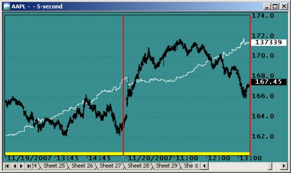
At this point you can scroll back and forth in time to see how BF volume differs from RT collected volume. Do not click CREATE, or you will overwrite the BF composite. The charts below show what your charts should look like.

Figure 5 – BF composite (Yellow) on BF Volume Histogram

Figure 5 above shows a period where the composite covered backfilled volume (for example the backfill period before RT collection). Because the composite copied this BF data, they match perfectly.

Figure 6 – BF Composite (Yellow) on RT collected Volume Histogram

Figure 6 above is for a period where the composite (backfilled volume) is superimposed on the real-time collected volume (histogram). Note the difference between the two types of data.

Developing a trading system should start with learning about the basics; delays and bad data quality can kill any HFAT trading system no matter how much time you spent developing it. The best way to understand and know what you are working with is to write a few small programs, like those that were included in this series.

Conclusion

In the previous discussions, it became clear that developing an HFAT trading system might not be as easy as you think. Googling for information will reveal very few links to practical information; you’ll be mostly on your own to discover the pitfalls. Developing with live data from your paper-trading account may be better than using backfilled data. However, since it is highly likely that IB executes paper trades subject to the reported price and volume you see, paper-trading results may not match actual trading results. Unless you are acutely aware of the various problems and can develop your system to work around them, it would appear futile to try and develop an HFAT trading system with 5-second IB data. The unique real-time volume patterns also occurred in data collected from the real-trading account.

Data from all sources will have their own unique problems, and it is prudent to perform some basic testing to get to know your RT data before spending considerable time on development.

Note

IB Snapshots and data compression methods are relevant to the above discussion; even though there isn’t much detail available, you may want to read the following threads to learn more about these topics.

AmiBroker user group: Interactive Brokers Plug-in dropping volume data
IB’s Discussion Board: Globex Ticks snapshot or reality?
AmiBroker User Group: AB Tick Bar Analysis

Edited by Al Venosa.

Filed by Herman at 6:28 pm under Real-Time System Design
Comments Off on High-Frequency Automated Trading (HFAT); part 2

Backfilled vs Real-Time Data issues

If you are not sure what HFAT (High Frequency Automated Trading) is all about, please Google the topic. This post highlights some of the problems you may encounter when venturing into HFAT of stocks. The views expressed here are based on personal experiences and/or may be anecdotal; not everything that happens in real-time trading is easy to explain. If you have technical insight and see inaccuracies, please comment for the benefit of future readers.

Designing and implementing high frequency trading systems is, from a trader’s viewpoint, probably the ultimate experience. To see and hear trades executed every few seconds and see the profits rolling in should give any trader an unprecedented high.

The catch is that to design an HFAT system that works with real money is very different from designing one using local data. The smaller the time frame the greater the impact of small data discrepancies. In sub-minute time frames, your HFAT system may perform very differently with local data than with real-time, raw market data.

A typical problem is that real-time live market data are delayed by up to several hundred milliseconds and that quotes may arrive out of sequence. What you see on your charts may be several quotes after the trade took place. This flawed data is what your trading system is trading and must be designed to work with. The charts you see in AmiBroker are mostly backfilled and/or updated after trading hours. At the end of a trading day, you will have data in your database that have a mixture of backfilled data (time and data errors have been corrected) and raw data (flawed) that were collected during the current day’s trading session. You may also have several lengthy data gaps that were introduced when you shut down the system and/or you lost your data feed.

While the procedure may vary for different data providers, quotes that are received in real time will lag in time. Since bar periods during live data collection are based on your computer clock, quotes may end up in the next bar due to their delayed arrival. The data used to backfill your database come from a different data server and will be time stamped. This allows AmiBroker to correct the position of quotes that were received out of sequence. This process removes the real time delays that were present when the data was received.

Since there are no delays with backfilled data, your backfilled data look ahead by several hundred milliseconds with respect to the data you will eventually be trading.

It is not unusual to develop a system with 5-second backfilled data (where all bad ticks and time-stamp errors have been corrected by the data provider) and obtain Holy Grail performance only to find out that when traded with real-time streaming data (where the data is delayed, contains bad ticks and time-stamp errors), the system is a total failure. The following charts illustrate this problem. The data to the left of the red line is backfilled and the data to the right of the Red line is data collected in real time. White is the equity.

You will not be able to visually judge whether data are backfilled or raw. The differences will only show up by running a trading system on the data; your trading system may be the only way to distinguish between backfilled and raw data. The chart below shows a close up of the data change.

Backfilling the above database and performing another Backtest over the same period produces a very different equity:

There is no guarantee that a system developed on one type of data will perform equally well with the other. When you first encounter a major equity drawdown, you may assume that this was just “a bad day”; after all, all trading systems have them. You may have developed and backtested your system over thousands of trades, covering a period of six months or more. You have been a good student and have used all the recommended methods to validate your trading system. You have tested in- and out-of-sample, applied intelligent optimizations, used Walk-Forward testing, performed Monte-Carlo analysis, and the list goes on. After being so thorough, how could you go wrong? You are ready to trade real money tomorrow and make your first 50% in one day!

The point is that all this effort is wasted time if the data used during development aren’t 100% identical to what you will be trading with.

The best way to develop an HFAT system is to use real live market data. The earlier you change from local or edemo data to real data, the more time you will save, and the more disappointments you will be spared. An HFAT system can never be completed off line, with a local database, or with simulated edemo Data. Its design must always include a significant paper trading and real-money phase.

Another problem when trading your IB paper-trading (simulated) account is that the user does not know the rules Interactive Brokers uses to decide whether an order should be executed or not. These execution criteria may change without warning. This imposes an artificial order to your executions that is unreal; the simulated market conditions will be different from those encountered in real trading. You may well develop a trading system that exploits IB’s way of processing to give you unreal performance, but such a system would fail in real trading.

Also, your paper-trades are not seen by, and cannot influence, the market. When trading real money your orders could be setting a new High or a Low, or if you are trading large sums, you could draw the price up or down. This means that even if your system performs extremely well in simulated trading, this is no guarantee that your system will perform well trading real money.

Using your simulated account to validate your system should never be your final validation before trading for profits; you should always include a real-money evaluation phase in your development plan. Your first real trades should never be to make money; they should be planned to validate your system under varied conditions.

Market behavior is very complex; be prepared for the unexpected and never skip a development step because something works extremely well. For example you might be testing your system using your IB simulated paper-trading account and see your profits skyrocket too fast to follow, perhaps having 90% winners and RARs that are out of this world. When this happens, it is extremely exciting and fun to watch; it is a rare experience that must be appreciated. It suggests that Holy-Grails are possible. But are they? Such favorable trading conditions may last for a few hundred trades, a few hours, or perhaps a few days. This can happen when technical conditions and market behavior are all just perfect for your system. Some unknown factor just made everything work perfectly. When you experience this, you’ll be analyzing your charts, trading log, execution report, etc. for weeks to follow. The fact is that it may never happen again, and you may never know what really happened.

Order and Position Status

IB Position size reporting may be erratic, is always delayed, and may include transient information. If you are trading fast and you use the IB Position Size to determine your next action, this will be a problem. This is especially the case with reversal systems where Covers may be processed before the Buys, and there may be many partial fills. For example, if you are reversing 100 shares, going alternatively Long and Short, you might read position sizes of 0, 100, 200, and even 300 shares. Do not base your system’s action solely on a single reading of the position size; your protective mechanisms will shut down your system many times a day. If a position is not what it is supposed to be on 5 consecutive queries (at quote interval), you may want to close all positions, suspend operation and continue later, or shut down the system and retry later.

Reporting of order status appears more reliable and stable. Usually it seems unnecessary to repeat Order Status queries.

IB Snapshots

Not addressed in this post is the matter of Snapshots however it is extremely important for real-time traders to understand how IB compresses and transmits its data. This topic has been discussed on several forums, for more information on IB data in general please read the following threads:

AmiBroker user group: Interactive Brokers Plug-in dropping volume data
IB’s Discussion Board: Globex Ticks snapshot or reality?
AmiBroker User Group: AB Tick Bar Analysis

The IB Maximum Message Rate

IB has a limit to the maximum rate of messages (order related) you can transmit per second. The rate of queries is not limited. The current limit is 50 messages per second. If you exceed this rate, IB will produce an error code, and if you continue to exceed the message rate, IB will suspend your connection. This, of course, should be prevented at all cost. The message rates are documented here. How to introduce real-time delays measuring in milliseconds is documented in the post on High Precision Interval and Delay Timing.

Internet Delays

Order and Position status is subject to a 50-400 milliseconds Internet delay. This delay will vary with your location and type of Internet connection to IB. You can test this delay by pinging the IB server. To do this type ping gw1.ibllc.com on command in the Start->Run windows (for Windows XP), and click the run button. A window, as shown below, will appear and show you the delays for three consecutive queries (pings) to IB:

If you encounter excessive delays or cannot connect at all, you can get more details about how your connection is routed by running tracert gw1.ibllc.com in the same manner. You may want to browse the Technical FAQ at IB for related items.

Edited by Al Venosa.

Filed by Herman at 8:55 am under Real-Time System Design
Comments Off on High-Frequency Automated Trading (HFAT); Part 1

This post shows how to add intraday session timing to the Real-Time Gap-Trading (RTGT) system developed in the previous post. However, before tackling session timing, there are a few things you should be aware about:

Time-Synchronization

In real-time trading there are many functions that are timed with reference to your system’s clock. It is therefore imperative that you always synchronize your computer clock with an Internet timeserver before each trading session.

Tools -> Preferences -> Intraday settings

Data Timestamps can be aligned to either the start or the end of the base period. The code developed here uses time of FIRST tick inside bar, i.e., the data timestamp returns the time at the start of the bar. This is when the first quote for the new period arrives and defines the Open for the new bar. Click Tools -> Preferences -> Intraday to set this option:

Backtesting and Bar-Replay

During backtesting the timing resolution will be equal to the periodicity set in AA Settings. If you are comparing Backtester signals with the signals displayed on your chart, you must make sure that the AA and Chart use the same periodicity.

During Bar Replay the timing resolution will be equal to the greater of the base interval of your database or the Step Interval selected in the Bar-Replay window.

During Backtesting and Bar-Replay, AmiBroker will refer to the timestamp to know how prices change over time. Hence, you will have no choice but to time events, such as session timing, with reference to the data timestamp.

Live Trading

When trading from an Indicator, the data timestamp is rounded to the selected chart-periodicity, i.e., if you display a 1-minute chart, the timing resolution will be one minute. This means you cannot implement delays based in seconds using the data timestamps of a minute database. This is why most functions in a real-time trading system use the computer clock as reference.

You can, with caution, use either the data timestamp or the system’s clock to control your session. However, since the data timestamp is dependent on the arrival of new quotes (ignoring data padding), using data timestamp could be unreliable. If you want higher timing resolution, you could create a 5-second database. However, this means working with slow backfills and slow AFL executions, due to lengthy data histories. To keep things simple, we will use a one-minute database.

Session Timing

When you are developing real-time trading systems, it is often handy, even essential sometimes, to develop several code versions. Typically, these might include:

1) A version for Backtesting and Bar-Reply. This version would use the TimeNum function for timing.
2) A Real-Time trading version. This version would use the system clock (Now()) for timing and would be highly optimized for AFL execution speed.
3) A DebugView version. This is a useful intermediate development stage that lets you run your system in real-time without any TWS interfacing; it logs trades to DebugView instead of sending them to the TWS.

ParamTime() input statements are used to set the start- and end-time of the trading session. The code below is only intended for preliminary system evaluation using the Backtester: hence, is uses time-numbers for session timing.

The StartOfSession and EndOfSession variables are triggers (they last only one bar). They are used to initialize processes at the start of the session and clean up processes at the end of the session. The InSessionTime variable is True during trading and is used to control processes that must be turned On/Off depending on whether you are trading or not. These processes will be covered in future posts.

A TimeFrame Parameter has been added to help visualize how the system works in different timeframes. To see the equity for different timeframes, just drag the slider to see the system response to any timeframe from 1 minute to 1 hour. Having added Session Timing you can now explore whether this system is more profitable during certain hours of the trading day. I suggest you perform an individual backtest on you favorite watchlist; you may be surprised to find that with some systems there is no need to trade all day. More…

For debugging purposes, you can turn On/Off a colored ribbon to display the Start- (Green), End- (Red) and In-Session (Yellow) variables.

For convenience the code below includes all previously developed parts. Just copy to an Indicator formula window, and click Apply.

<p>_SECTION_BEGIN("SESSION TIMING"); 
<p>TimeFrame= Param("Chart Timeframe (min)",1,1,60,1)*60; <p>TimeFrameSet(TimeFrame); <p>TN = TimeNum(); <p>ParamStartTime = ParamTime("Session Start","09:30:00"); <p>ParamEndTime = ParamTime("Session End","15:59:00"); <p>InSessionTime = TN &gt;= ParamStartTime AND TN &lt;= ParamEndTime; <p>StartOfSession = InSessionTime &gt; Ref(InSessionTime,-1); <p>EndOfSession = InSessionTime &lt; Ref(InSessionTime,-1); <p>InsessionTime = InSessionTime OR EndOfSession;
<p>_SECTION_END();

<p>Buy = O &lt; Ref(L,-1) AND InsessionTime; <p>BuyPrice = O; <p>Sell = L &lt; Ref(L,-1) OR EndOfSession; <p>SellPrice = C; <p>Short = O &gt; Ref(H,-1) AND InsessionTime; <p>ShortPrice = O; <p>Cover = H &gt; Ref(H,-1) OR EndOfSession; <p>CoverPrice = C; <p>SetTradeDelays(0,0,0,0); <p>SetOption("CommissionMode",3); <p>SetOption("CommissionAmount", 0.005); <p>E=Equity(1); <p>TradeEquity = ValueWhen(Sell OR Cover,E); 

<p>_SECTION_BEGIN("PLOTTING");
<p>Plot(C,"",1,128); <p>if( ParamToggle("Session Timing Ribbons","HIDE|SHOW",0) ) <p>{ <p>Plot( InSessionTime,"",7,styleArea|styleOwnScale|styleNoLabel,0,60); <p>Plot( StartOfSession,"",5,styleArea|styleOwnScale|styleNoLabel,0,30); <p>Plot( EndOfSession,"",4,styleArea|styleOwnScale|styleNoLabel,0,30); <p>} <p>OutOfSessionColor = ParamColor("Out of Session",colorDarkRed); <p>Plot(NOT InSessionTime,"",OutOfSessionColor,styleArea|styleOwnScale|styleNoLabel,0,1); <p>PlotShapes(IIf(Buy, shapeSmallUpTriangle, shapeNone),5,0,BuyPrice,0); <p>PlotShapes(IIf(Sell, shapeHollowDownTriangle, shapeNone),4,0,SellPrice,0); <p>PlotShapes(IIf(Cover, shapeHollowUpTriangle, shapeNone),5,0,CoverPrice,0); <p>PlotShapes(IIf(Short, shapeSmallDownTriangle, shapeNone),4,0,ShortPrice,0); <p>if(ParamToggle("Equity curve","HIDE|SHOW",0) ) <p>{ <p>Plot(TradeEquity,"",2,styleStaircase|styleOwnScale); <p>}

Filed by Herman at 2:07 pm under Real-Time System Design
Comments Off on Gap-Trading demo, Session Timing Example

This system was intended to provide signals to demo trade automation. However, its signals are not that frequent and it proved to be quite boring to automate it. The code is left here but I plan to use another system to demo trade automation. You may also note that I separated Real-Time System Design from System Automation. This was done to allow categories to evolve independent from each other.

To develop trade-automation code we need a demo system to generate signals and to test TWS interfacing. To be able to continue this series and not waste time looking for a superb system, I’ll use the following very simple trading rules:

Buy at the Open of the current bar if it falls below the previous Low.
Sell at the Close when the current Low falls below the previous Low.
Short at the Open when the Open exceeds the previous High.
Cover at the Close when the current High exceeds the previous High.

In AFL this looks like this:

SetOption("CommissionMode",3);
SetOption("CommissionAmount", 0.005);
SetTradeDelays(0,0,0,0);
Buy = O < Ref(L,-1);
BuyPrice = O;<br>Sell = L &lt; Ref(L,-1);
SellPrice = C;<br>Short = O &gt; Ref(H,-1);
ShortPrice = O;<br>Cover = H &gt; Ref(H,-1);
CoverPrice = C;
E=Equity(1);<br>Plot(C,"",1,128);
if( PlotTriangles = ParamToggle("Triangles","HIDE|SHOW",1) )
{
PlotShapes(IIf(Buy, shapeSmallUpTriangle, shapeNone),5,0,BuyPrice,0);
PlotShapes(IIf(Sell, shapeHollowDownTriangle, shapeNone),4,0,SellPrice,0);
PlotShapes(IIf(Cover, shapeHollowUpTriangle, shapeNone),5,0,CoverPrice,0);
PlotShapes(IIf(Short, shapeSmallDownTriangle, shapeNone),4,0,ShortPrice,0);
}

The above code is a variation of The Full Gap-Trading system. You can read more about this type of system on the Stockcharts site and many other Internet sites.

This system will produce trades in all timeframes, trade frequently, and trade both long and short. Running this system in the 1-15 minute timeframe will give us lots of action and make it easier to develop and debug the Trade-Automation (TA) code. An AT trading system designed around a system that gives only a few signals a day will take forever to debug. Mechanical performance is the first objective.

For now we assume that we can enter at the bar’s Open price. Note that I exit at the Close of the bar because, in the AmiBroker database, this is the next price that is available. At this stage this system is designed to stimulate trade-automation code and not to make you rich; DO NOT TRADE IT. Order types and/or strategies will be decided on later. Trade-Delays are set to zero because they are better handled in the code. The Equity(1) statement is used to remove redundant signals. The indicator should display trades as follows:

Edited by Al Venosa.

Filed by Herman at 5:00 pm under Real-Time System Design
Comments Off on Real-Time Gap-Trading Demo, Basics (v3)

The phenomenon that is the basis of many trading systems is the observation and trading of an exceptional price movement followed by a pullback.

An extreme example of the pullback phenomenon would be a Spike as shown in the chart below. Because the price change is so extreme, the pullback or correction appears instantaneous. There is no clear market response, i.e., traders at large are not inclined to take the price change seriously.

The problem is that inadvertently you can easily write code that trades these spikes. Only when you start trading such a system will you discover that your orders are not filled because the volume just isn’t there. This is a common reason why backtested and real results may sometimes differ substantially. You may have designed a system that is completely rational, backtests perfectly, and stands up to the most detailed technical scrutiny, only to find out that in real trading it fails completely.

You might think that by increasing the timeframe, for example to 15-minute or even daily, you can minimize this problem. However, while doing this may make the spikes less prominent, the tradability will not improve. Consider the spike in the 15-minute chart below:

Adding a few percent bands makes this look like a real trading opportunity. It looks so easy! However, the Low of the bar is still created by a single trade and the chance to get your order filled would still be minimal. Designing trading systems around minimal-volume price changes is one of the easiest traps for a real-time system developer to fall into. When designing an intraday trading system you should design your code to minimize the divergence of the backtester with respect to real-trading results. You can do this by working in the smallest time frame possible. Even when trading at hourly intervals you should write your code in the minute (or even Tick) timeframe.

There are a number of ways in which to do this. Take a look at the 10:30 AM spike in the 15-minute chart below and consider how you would determine its tradability:

The fact is that there is no way to tell whether the 10:30 AM High is tradable. However, expanding the chart to the 1-minute timeframe, as shown below, lets you clearly see a gradual reversal pattern. This means your order could probably have been filled somewhere near the top of the 15-minute spike shown earlier.

Running your Backtester in the 1-minute timeframe and looking for one-bar confirmations may drop your backtester performance, but your results would have been closer to that which can be obtained in real trading. In this case you would have separate Backtester and Trading code versions for your system; the Backtester code would include signal confirmation while your Trading code would not.

Edited by Al Venosa.

Filed by Herman at 6:07 pm under Real-Time System Design
Comments Off on Designing a Tradable System – Spikes

When you are designing a real-time trading system, many things can go wrong. This post is intended to alert you to some of the potential pitfalls. However, that is all it can do. Only experience can teach you how to prevent them. Be aware that even the most experienced designers will make some of these mistakes repeatedly.

Since documenting all potential pitfalls with coding examples would consume too much time and space, they are, for now, only briefly commented on. Most of them will trigger a user response of “Oh yeah, that happened to me!”. If you need a more detailed explanation you can post questions in a comment to this post

No rules exist to prove that a trading system is free from coding or logical errors. However, two indicators are fairly reliable in suggesting you may have a problem:

1) Your profits are simply too good to be true. In this case you have no choice but to work through the code line by line, trying to find lines of code that look into the future. If that doesn’t reveal any errors, then you would have to inspect the plotted signals and trade list trade by trade.
2) Your system is very profitable trading Long but not Short, or Short buy not Long. When this happens, you may have an error in either the Long or Short parts of your code, and comparing the two sections will often reveal the problem (this only works for reversal systems). However, it could also be that your code is correct but that your trading principle is overly trend sensitive. This would almost certainly get you in trouble when the trend reverses. In this case no other cure exists than to re-think the basic system.

When designing high-frequency trading systems, i.e., those whose trade durations are in minutes, everything changes, and many traditional procedures fall apart. Internet delays, data delays, bad data (spikes), temporary system freezes (Windows sometimes has a mind of its own!), lagging status reports, TWS problems, etc., all become critical issues that will prevent you from obtaining a close match with the Backtester.

Many of these problems will only surface when you start trading real money. Hence, the final stages of developing a trading system should always involve trading real money. Here is where the Interactive Brokers account simulator (paper-trading account) may be an indispensable tool since you can test your system in real time without committing real dollars. But, since the market does not see your trades, even paper-trading results will differ from trading real money. In general, the faster you trade, the greater your real-trading results will deviate from your backtest results. You should also be aware that commissions play a much greater role on performance of high-frequency trading systems because trade profits are smaller.

No matter how you go about it, troubleshooting a complex trading system will almost always be a tedious and boring job that could keep you busy for several days or weeks. If you find that certain problems continue to resurface, they are likely related to your personal development style, and you may be able to write some code that checks for these specific problems. See the Debugging category for some ideas.

The list below, which is not exhaustive, is presented to caution you that many areas can lead to problems. Some are obvious, while others may be expanded on as needed and time allows.

– High/Low precedence (contrary to EOD where the Backtester is unable to determine which came first, the entry/exit or the high/low, in realtime there can be no ambiguity in price precedence).
– Data Delays (real-time data may be delayed for various reasons and time periods (Internet delays, lack of quotes, packets vs. ticks, etc.).
– Low Liquidity (there may be no-volume trading periods).
– Data Holes (bars with no trades).
– Data Spikes (high spikes without volume may trigger trades).
– Data Padding (a bar without data may be padded).
– Premature Padding (the last bar may be a padded bar).
– Data Accuracy (prices you receive aren’t always accurate).
– Random Slippage (you will rarely get the expected price).
– Breakout slippage (you will rarely get the Breakout price of your system).
– Survivorship Bias (companies that didn’t do well and stopped trading won’t be in your database, i.e., you are working above average stocks).
– Lucky Trades (a series of lucky trades may look like good performance).
– Parameter Over-Optimizing (optimized parameters are rarely stable over time).
– Design Over-Optimizing (frequent testing is like running an optimization and may be leading to false conclusions).
– Out–of-Bound Prices (with PriceBoundChecking turned ON, AmiBroker forces the trade price within the High-Low range, this may hide pricing errors).
– Price Rounding (prices may be rounded or truncated by the broker).
– Wrong Use of >= and <= (when using both <= and >= in the same statement, only the first equal condition will ever be seen).
– Comparing Floating Point Numbers (calculated values can have many decimal places, either round values or use the AlmostEqual()).
– Chart Justification (make sure you are looking at the Last bar!).
– System Mortality (no system will work forever).
– Sharing Trading Systems (sharing systems with other traders may result in over-trading a system).
– Being Duped by a Trend (a rallying ticker may make your system look like the HG (holy grail).
– Tricking AmiBroker (AmiBroker has its limits; it is possible to write esoteric code that will produce wrong results).
– Order Visibility (placing your order for every trader to see may influence the orders they place).
– Making the Market (extreme example: if you place a MKT order during a no-trading period you will change the chart).
– Window/Pane Execution Order (when passing variables between panes or windows do not assume that they execute in a fixed order, more).
– Trading at the Open (order execution at the start/end of day is different from midday because of volatility and data delays).
– IB Data Snap Shots (snapshots are only representative of prices traded).
– Trade Delays (make sure you understand your trade delays when backtesting).
– EOD and Intraday Gaps (There is no time interval in RT gaps).
– Time Zones (make sure your computer and database timezones are properly set).
– Very Short Time-Frames (prices jump and are less contiguous).
– Setting LMT Prices (consider rounding for faster order executions).
– 24-Hour vs. RTH (Regular Trading Hour) Backtesting (extended hours can rarely be traded like RTH due to huge bid/ask spreads and low volume).
– Static Variables Naming (use unique names for your static variables).
– Incorrect Computer Time (computer time offset from market time can cause real problems).
– Look-Ahead Problems (not all look-ahead coding problems are obvious).
– Buy/Sell Precedence in a Loop (be aware that AB and custom AFL loops enforce a Buy/Sell priority).
– RT Candle Discrepancies (RT Candles may be different from later backfills, especially in the opening print).
– Bars Loaded (consider bars-loaded with respect to execution speed and loops).
– Signal lifetime (signal strength quickly decays over bars in high frequency trading).
– SameBarExits (Sell signals may act as a qualifier for Buy signals).
– Designing systems based on High and Low triggers (these may fill in the Backtester but not in real trading). more…
– Using the wrong CommissionMode and/or CommissionAmount can make any system look good, or bad…
– Using zero TradeDelays is OK if you code the delays in your system’s code, else you may be looking into the future.

Edited by Al Venosa

Filed by Herman at 6:25 pm under Real-Time System Design
Comments Off on System-Design Pitfalls

Developing trading systems is a very personal activity, and opinions vary widely regarding what is the best approach. Most of the solutions presented here were developed by Herman van den Bergen. They may not be compatible with your personal preferences and you are encouraged to explore other alternatives more suited to your own trading style before deciding on a possible solution. To develop a Real-Time Automated Trading (RT/AT) system, you must have a trading system to automate. If you haven’t developed one yet, you may find some ideas in the Research and Exploration or Trading-Systems categories.

Modular design, readability, and simplicity of the system code are desirable to facilitate future maintenance. Posts in this category will progress through the various phases of developing a Real-Time Automated system.

Edited by Al Venosa

Filed by Herman at 8:58 pm under Real-Time System Design
Comments Off on Introduction to Real-Time System Design