Users' Knowledge Base

This page is obsolete. Current versions of AmiBroker feature built-in non-exhaustive, smart multithreaded optimizer and walk-forward engine.

As stated previously IO Directives will by definition be seen as comments by AB / AA / AFL and are thus unintrusive.  Below is a simple AFL with the required IO Directives in it.

ShrtLen    = Optimize("ShrtLen",         2,     0,   500,     1);
LongLen    = Optimize("LongLen",       304,     0,   500,     1);
UpPct      = Optimize("UpPct",        0.01,     0,    10,  0.01);
DnPct      = Optimize("DnPct",        0.36,     0,    10,  0.01);

ShrtAMA = AMA(C, 2 / (ShrtLen + 1));
LongAMA = AMA(C, 2 / (LongLen + 1));

if (ShrtLen < LongLen)
{
    Buy     = Cross(ShrtAMA, LongAMA * ( 1 + UpPct / 100 ));
    Sell    = Cross(LongAMA * ( 1 - DnPct / 100 ), ShrtAMA);

    Short   = Sell;
    Cover   = Buy;
}

That’s right … There aren’t any required directives. 

IO was meant to be a tool for USERS.

All the IO Directives are optional as they all have default values, all of which with a few notable exceptions I have set to what I believe the best settings to be are.  As a result there is no learning curve to climb in order to run IO. 

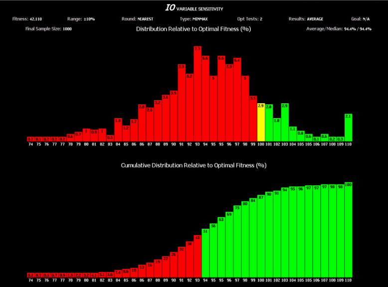
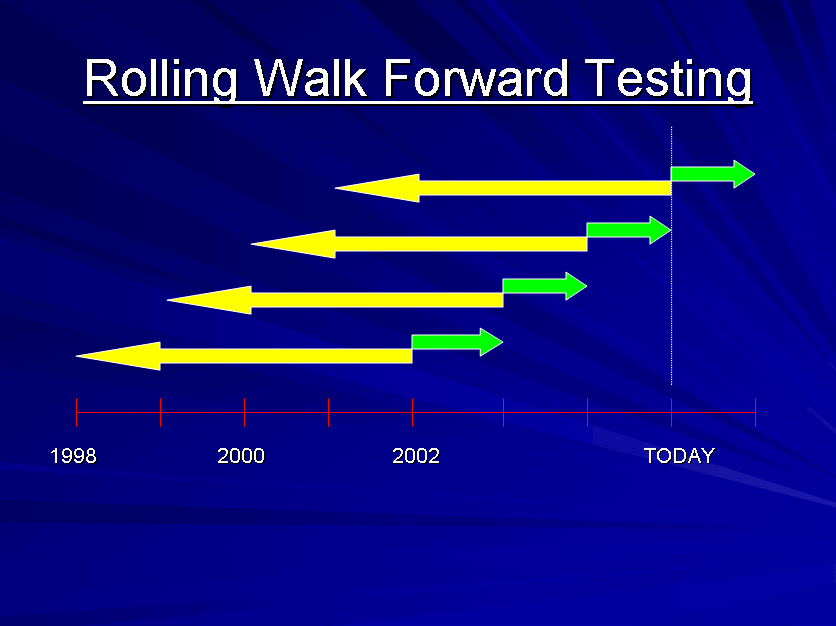
Getting the most out of IO by utilizing sensitivity testing during in sample optimization and performing walk forward testing does require knowledge of how to write those directives which anyone should be able to get up to speed on in a few minutes.

Initial setup of IO involves copying the IO Tasks.hta, IO.exe and IO.ico files from a zip to your AmiBroker directory.  Following that one would want to set up easy access to the IO Task Bar as it is the control center for all IO operations.  This can be from the AmiBroker, Tools, Custom menu or from the Windows Desktop or Quick Launch Bar ( My preference because its a single click ).  Once that’s established, clicking on the icon for the IO Task Bar will bring it up in the top left corner of the screen typically overlaying the AmiBroker title bar.  It can of course be moved to wherever the user desires.

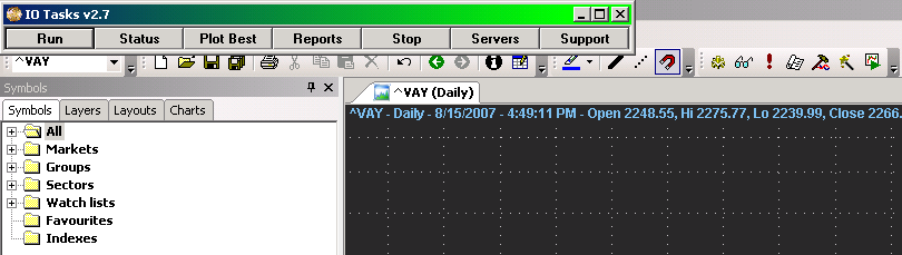
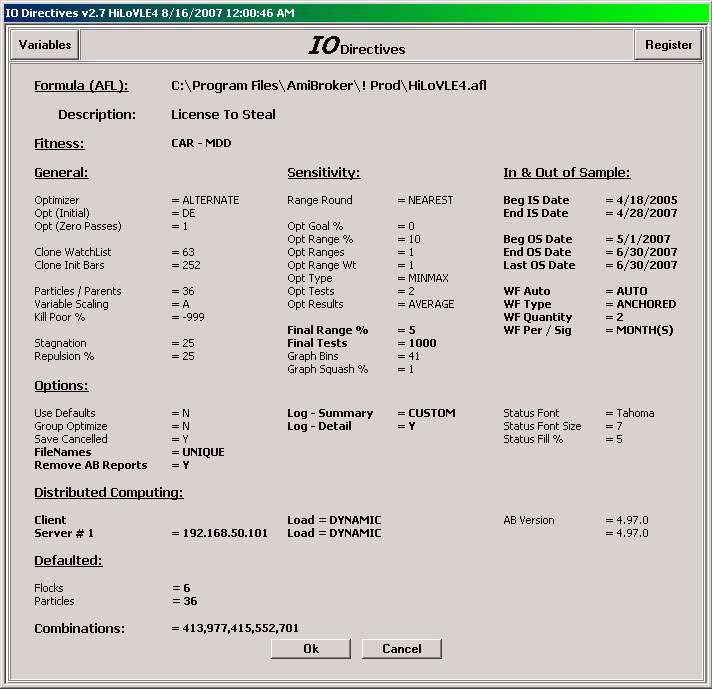
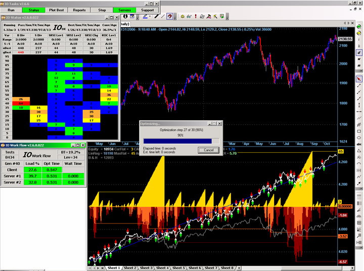
Clicking RUN on the IO Task Bar will start an IO run much like clicking Optimize in AB/AA or FE would start a regular AmiBroker optimization.  When IO begins it will first show the user the values for all the IO Directives, with the ones not having default values being in bold.  This provides the user a chance to review the directives and cancel the run prior to its beginning if modification to some directive is desired.

Once the user clicks OK on the Directives screen, optimization begins.  What one would see during optimization is short bursts of the AB Optimization progress bar which will appear, run to completion, disappear and then repeat.  IO is only active for very short spans of time, typically a fraction of a second, between the time that the AB Optimization progress bar disappears and when it reappears. 

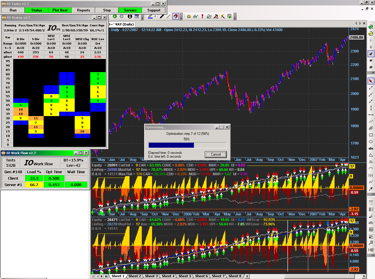
Other options from the IO Task Bar while IO is running are …  

    –    Status – Shows the status of the run ( Shown Above )

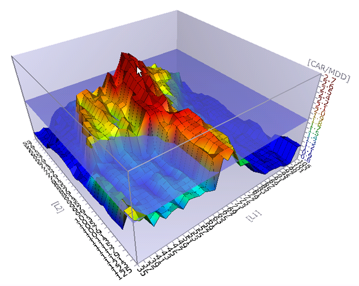
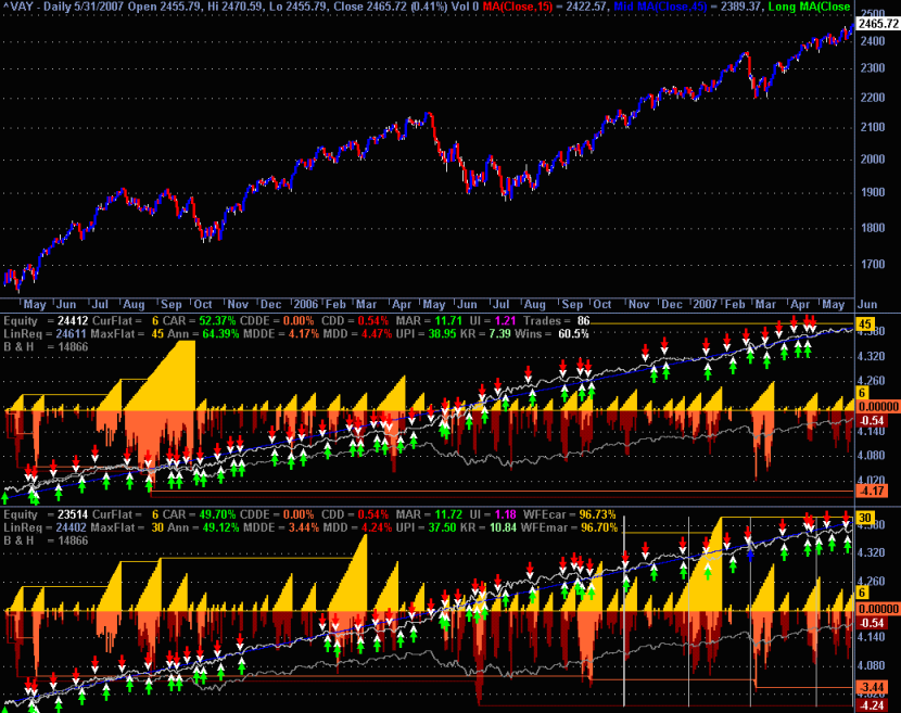
    –    Plot Best – Will automatically update an Equity Curve ( AB’s, Yours or Mine ) as new best solutions are found

    –    Stop – Will allow the run to be paused or cancelled

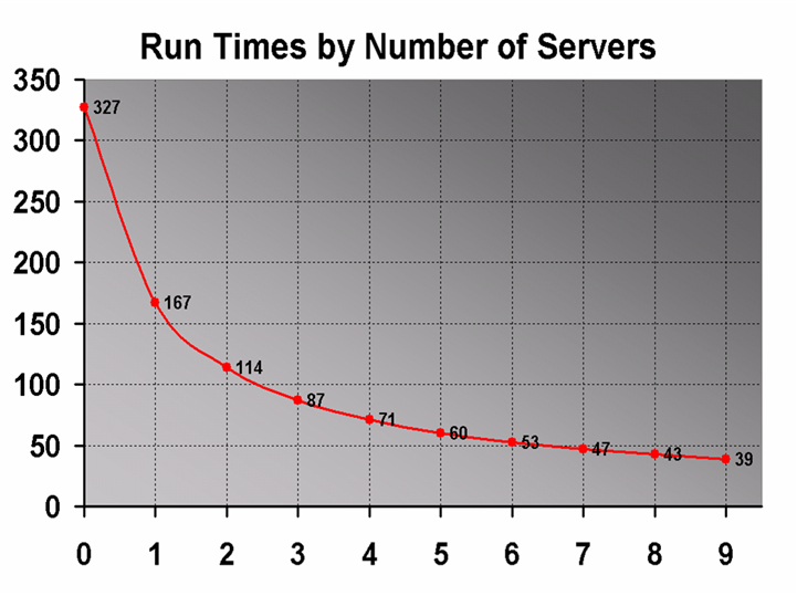
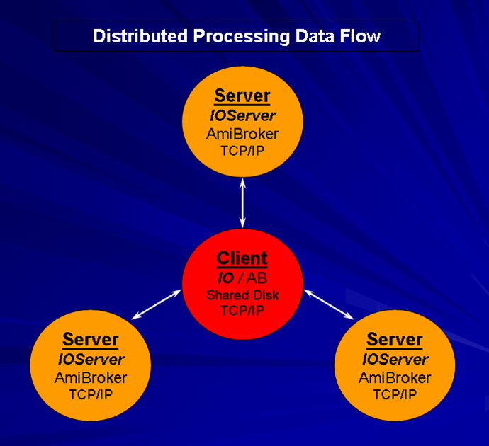
    –    Servers – Shows the Work Flow between client and server(s)  ( Shown Above )

IO Task Bar On/Off Type Buttons will change color when activated as shown above.  When a run is completed the equivalent of clicking the Reports button will occur which is to provide GUI access to all the Reports and Screens relative to the current and previous runs.    

This is the initial screen that will display:

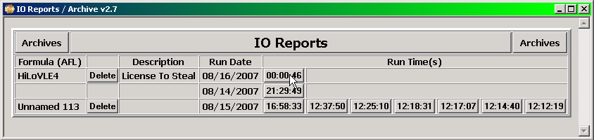
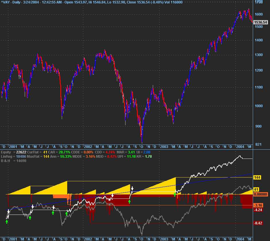
When an individual button relating to an IO run for an AFL for a specific run date and time is clicked then the summary for that run will appear. 

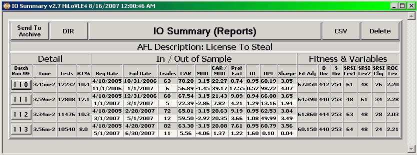
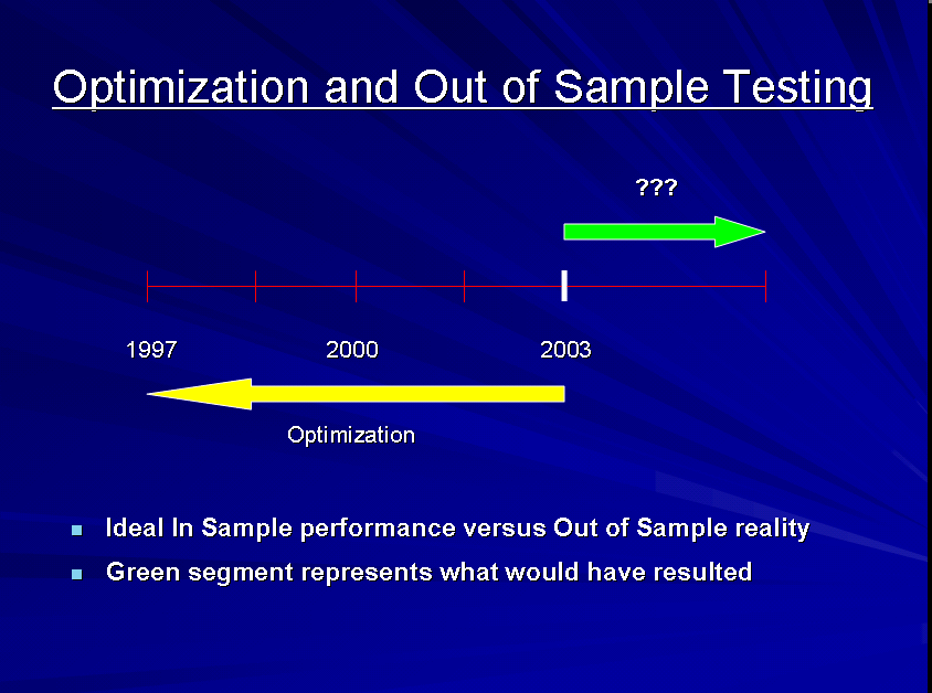
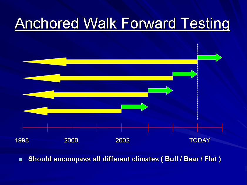
This typically shows the amount of time the run took and the number of tests performed along with whatever performance metrics the user desires as well as the parameter values of the best solution from optimization.  If Out Of Sample testing was performed then there will an additional line of performance metrics for the out of sample period.  If Walk Forward testing was performed then there will be multiple groups of the above information i.e. one for each Walk Forward segment.  Clicking on a button for a particular segment brings up a detail screen which shows the chart as of the end of that particular segment, the trade list for the in and out of sample period it covers and the result of final sensitivity testing. 

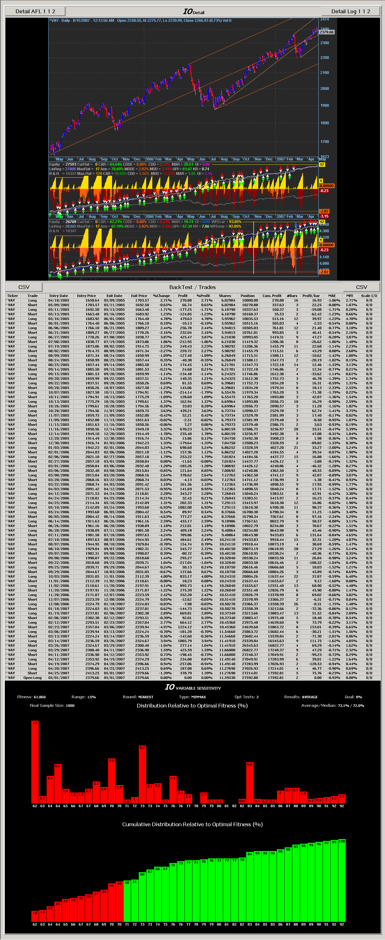
The Detail Screen has buttons to:

    –    Open a CSV file of the Trades, assumedly in Excel, for further manipulation if desired

    –    Show the AFL in play with the parameter values from optimization put into the default values of the optimization statements

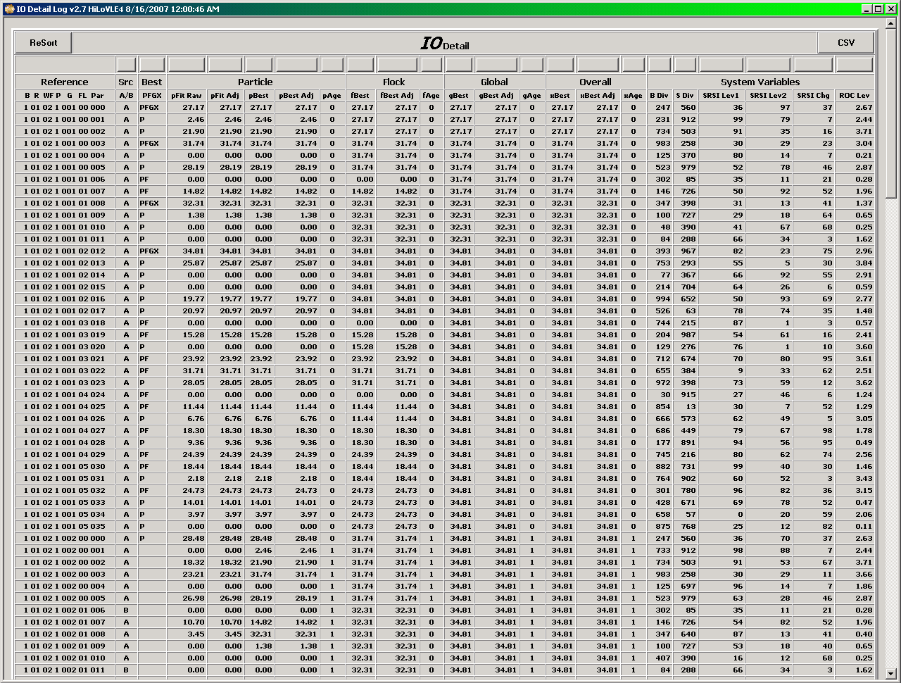
    –    Show the Detail Log if requested by IO Directive which will show the results of every test performed during optimization and can be sorted in any order desired.

A shareware version of IO with full documentation can be found in the AmiBroker Files Section …
http://groups.yahoo.com/group/amibroker/files/IO.zip
http://www.amibroker.org/userkb/wp-content/uploads/2007/08/io-reports.png

Filed by Fred at 11:11 pm under Intelligent Optimization
Comments Off on IO – Ease of Use

This page is obsolete. Current versions of AmiBroker feature built-in non-exhaustive, smart multithreaded optimizer and walk-forward engine.

The Objectives of an Intelligent Optimizer should include the ability to:

1. Optimize systems that would take too much time or would otherwise not be feasible using an Exhaustive Search approach. 
2. Optimize systems based on any user derived combination and/or relationship of the performance metrics provided as a result of the AmiBroker optimization process including those that users develop using the custom back tester and it should allow users to define Goals and Constraints that help direct optimization.
3. Perform a sensitivity analysis of the variables that have been optimized and utilize parameter sensitivity as a means of directing the optimization process towards a more robust set of parameters.
4. Perform automated out of sample and walk forward testing i.e. repeated cycles of optimization of in sample data followed by back testing of out of sample data using either a front anchored or rolling window.
5. Utilize distributed computing i.e. multiple machines to spread the optimization load over, thereby facilitating significantly faster run times.
6. Utilize the full capabilities of an Intelligent Optimizer even when the decision is to strictly use AmiBroker’s Exhaustive Search optimization engine.
7. Set up and solve more advanced problems not initially thought to be in the realm of optimization such as system generation via automated rule creation,  selection and combination; pattern recognition and data mining.

Besides having the above functionality … It should be Easy to Use …

It should be noted that if your AFL’s use constants instead of optimizable parameters that the values of those “constants” in many situations originated by someone else optimizing something manually or otherwise at some other point in time and as such only appear to be constants.  In addition as constants they have a tendency to hide how sensitive they are and as a result how robust or not the corresponding system they are part of is.

A shareware version of IO with full documentation can be found in the AmiBroker Files Section …
http://groups.yahoo.com/group/amibroker/files/IO.zip

Filed by Fred at 5:54 am under Intelligent Optimization
Comments Off on Intelligent Optimization – An Introduction

This page is obsolete. Current versions of AmiBroker feature built-in non-exhaustive, smart multithreaded optimizer and walk-forward engine.

The main factors involved in how much time optimizations take typically include:

.    The Number of Combinations of Parameter Values

The AmiBroker engine is the fastest I’ve ever seen but even with very simple systems like a MACD or Stochastic utilizing 3 variables with potential values ranging from 1 to 100 it can take a long time using an exhaustive search process.  The number of combinations for a simple system like this is 10 ^ 6 and even if our engine is capable of processing 100 combinations per second it will take close to 3 hours to complete the optimization process.   Using the same fast AmiBroker engine to repeatedly perform small bursts of optimization with a few ( 15 – 50 ) combinations per burst and then intelligently redirecting optimization based on the results will typically perform a task like this in 5 – 10 minutes.  For intelligent algorithms it makes little difference whether there are 3 variables to be optimized or 30 as this is not typically a factor that affects how long it takes them to solve problems.  Robust solutions to engineering problems with hundreds of variables are typically solved by intelligent algorithms as these are the only methods feasible.
The benefits here are that not only do intelligent algorithms allow us to run common optimization problems much faster; they also allow us to solve problems that would not otherwise be possible.

·    The Length of the Data Streams

One of the things I have observed over the course of time is that there is a distinct difference of how long operations in AmiBroker take depending on the length of historical data loaded in AmiBroker.  Changing the AA date range will have a minor effect on run times but we can have a much greater effect by cloning only the data needed from an existing symbol to a pseudo or cloned  symbol and using the clone for optimization.  As can be seen from the chart below, changing the AA dates to use only half the data results in a decrease of relative run times from 43 to 36 or about 16%.  However,  cloning the symbol with only half the data under a new symbol and using the clone for optimization results in a decrease of relative run times from 43 to ~25 or about 41%.  That’s a 25% difference between the two methodologies.

While at first glance this would seem painful to utilize, if we have the means to automatically clone only the historical data needed then we can significantly reduce run times that much further.  IO performs this function automatically. 

·    The Number of Data Streams

This includes the number Foreign symbols that are referenced as well as other issues like the length of Watch Lists etc. that are to be processed, neither of which we can have much affect on.

These are standard shareware features in IO.

A shareware version of IO with full documentation can be found in the AmiBroker Files Section … 
http://groups.yahoo.com/group/amibroker/files/IO.zip

Filed by Fred at 5:49 am under Intelligent Optimization
Comments Off on IO – Exhaustive Search .vs. Intelligent Algorithms

This page is obsolete. Current versions of AmiBroker feature built-in non-exhaustive, smart multithreaded optimizer and walk-forward engine.

In AmiBroker we have the capability to sort the results from optimization in AA based on any number of columns of performance metrics that are returned to us from the process but what if we want to be able to: 

·    Prioritize the results based on some combination of performance metrics written as an equation without having to use the custom back tester which while very capable does have an impact on run time 

If we could optimize systems based on the results of equations, which I will term Fitness, that we can write outside of normal AFL then this leaves us the flexibility to optimize on virtually anything without having to constantly rewrite potentially complex segments of code in the custom back tester.  As examples we should be able to optimize for Fitness based on simple expressions like: 

     –    Fitness = CAR / MDD ^ 1.5 

           Which allows us to value having a low MDD more highly then having a high CAR

     –    Fitness = CAR * 0.98 ^ Trades / MDD 

           Which allows us to value solutions with fewer trades as being more important 

     –    Fitness = UM1PH * CAR / MDD 

           Which allows us to incorporate a User Metric from the custom back tester in conjunction with other standard AmiBroker metrics 

·    Penalize potential solutions because they don’t meet certain Goals or Constraints we have such as having CAR that is too low or number of Trades that are too high for an intermediate term system we are trying to develop.  This would allow us to write and have optimization utilize statements like:

     –    Goal = CAR > 30

     –    Goal = Trades: < 50

     –    Constraint = MDD < 10

These are standard shareware features in IO.

A shareware version of IO with full documentation can be found in the AmiBroker Files Section …
http://groups.yahoo.com/group/amibroker/files/IO.zip

Filed by Fred at 5:45 am under Intelligent Optimization
Comments Off on IO – Fitness, Goals and Constraints

This page is obsolete

Almost all who have been trading for more than a short while have come to realize that without additional information, In Sample Optimization results are purely for bragging rights and as such have very little predictive capability for how some system is likely to perform where it counts … Out of Sample. 

One of the important pieces of information we can utilize to have some clue as to whether or not a system is likely to perform well out of sample is to take a look at how sensitive the parameter values we have chosen are.  With a two parameter system we can in AmiBroker optimize the system using traditional methods and then look at the 3d surface area plots that put the two parameters on the x and y axis and some performance metric on the z axis like in the chart below.

As in the chart above it is not uncommon for the highest peak to be immediately next to an area where system performance falls off significantly.  The parameter values representing this peak then could be referred to as being too sensitive or not particularly robust.  While this might be a very good system we would not want to use the parameter values that put us right at that peak as the probability of failure or at least significantly different results in real trading is too great.  We would want instead to select parameter values that while still performing well In Sample also had a higher probability of performing well Out of Sample because they weren’t as sensitive.  This could be illustrated by where I’ve placed the arrow in the above chart.

While the 3d surface area plots in AmiBroker are fine for visualization of Sensitivity and then to at least some degree Robustness with 2 parameter systems, they won’t help when one is trying to understand the Sensitivity of parameter values with systems that have 3 or more parameters.  One way to have some idea of how sensitive the parameter values are with systems that have 3 or more parameters is to take a statistically significant number of points and randomly generate values for each of the parameters that represent those points in some percentage range that is plus or minus from the original point, test those for fitness and then compare the results to the fitness of our original point.  For example in the above chart let’s assume that the parameter values for L1 and L2 as represented by where I placed the arrow are at 75 and 70 respectively and we chose for our range to randomly test other points in the +/- 5% range. We could then test points with values for L1 varying from ~71 – 79 and for L2 varying from ~66 – 74.  This would give us data that could then be plotted in a different way that showed us how sensitive those parameters are.  Below is an example of such a plot using a bar chart to categorize groups of points and their fitness relative to the fitness of our original parameter values found in optimization.

The top section of the chart shows categories and percentages of points tested and for example the tallest bar shows that 7.3% of the points tested had fitness that was 93% as good as our original point.  Also notice that since the fitness of the original point we picked was not the highest peak in the original 3d surface area plot, that some bars in the chart above have a higher than 100% value.  The bottom section of the bar chart is composed of cumulative values from the top section and for example shows that 45% of our tests were less than 93% as good as our original point.  While this tool may not appear to be quite as useful as the surface area plots, keep in mind that it is valid regardless of the number of parameters being optimized. 

The above are standard shareware features in IO.

Given that unlike Exhaustive Search an Intelligent Optimization methodology will by its nature not examine every possible combination of parameter values, it would be unlikely without some additional influence or direction that the Intelligent Optimization process would have picked for parameter values those that were not particularly sensitive.  This is because the processes of judging or calculating parameter sensitivity are typically performed after the optimization was finished because with Exhaustive Search that is all that is required as we had a chance to view the results of all combinations.

In order to ensure that parameter sensitivity is taken into account when looking for parameter values with high fitness utilizing an Intelligent Optimizer, it is necessary to have a methodology for evaluating how sensitive parameter values are and to have that in turn impact the fitness calculation during the optimization process so that the process is led to a more robust set of parameter values.

Given that the Intelligent Optimization process as implemented in IO sends parameter values to AmiBroker for evaluation by its optimizer and retrieves results back from AmiBroker to determine how it should alter its search pattern in the next generation, this is more straight forward then it would first appear.  This is accomplished by between one generation of regular optimization and the next looking at the results coming back from AmiBroker and for those points that are worth further examination performing some tests for Sensitivity that are not dissimilar to the methodologies used to generate the bar charts above.  The IO options and mechanics for this while not difficult for the user to employ are varied and fairly sophisticated and as such rather than discuss all of them here I would recommend for those who are interested that you read the sections on Sensitivity in the full documentation.

The above are advanced features in IO.

A shareware version of IO with full documentation can be found in the AmiBroker Files Section …
http://groups.yahoo.com/group/amibroker/files/IO.zip

Filed by Fred at 5:43 am under Intelligent Optimization
Comments Off on IO – Robustness, A Sensitive Subject

This page is obsolete. Current versions of AmiBroker feature built-in non-exhaustive, smart multithreaded optimizer and walk-forward engine.

As a more thorough verification that a system will perform as anticipated, we should always test the system with out of sample data or in other words with data that has not been seen by the In Sample optimization process graphically represented by:

This can be accomplished in AmiBroker by:

    –    Setting the from and to dates for our system to wherever we want

    –    Performing an optimization and choosing the parameter values to use going forward

    –    Changing the default values of the optimization statements

    –    Moving the from and to dates forward in time

    –    Running a back test to see how well the system performs.

Besides automating the whole process above, IO also offers more advanced alternatives such as a fully automated calendar or signal based, anchored or rolling Walk Forward optimization and Out of Sample testing which can be made to be very thorough.  Graphically the anchored and rolling walk forward processes look like this:

Without automated tools such as this almost no one performs Walk Forward testing because of the amount of manual intervention that is required.  For example think about the manual steps required to perform a Walk Forward test over a 3 year period 3 months at a time which are:

    –    Set the from and to dates for the original optimization to begin as of some date in time and end as of 3 years ago

    –    Perform the optimization and choose which parameter values to use going forward

    –    Change the default values of the optimization statements

    –    Move the from and to dates forward

    –    Run a back test for the first three months of out of sample data and record the results

    –    Then repeat the whole process eleven times, each time moving the end date ( anchored ) or beginning and ending dates ( rolling ) 3 months closer until you run out of data.

Assuming one had the means to manually stitch together the out of sample equity curve this then would provide a real life picture of how the system performed over a 3 year Out of Sample period with reoptimization occurring every 3 months.

The above can be accomplished in IO with no manual intervention and a single Walk Forward Directive which is written like this:

    –    WFAuto: Anchored: 3: Months 

As a result even if it takes 15 minutes to optimize each of the 12 segments to accumulate the data necessary to build and show the tables and the combined equity curves, it can all be done unattended.  As a result one only need to set up a run, get it started and then go find something else of interest to do.  Besides the tabular results that are produced by IO it is also capable, with an included AFL, of showing an accurate composite of the In and Out of Sample equity curve in AmiBroker that looks like what is below:

The middle pane in the template above shows my replacement for the standard AmiBroker equity curve for the current In Sample optimization.  The bottom pane shows the full Walk Forward results and is constructed on the fly as each new Walk Forward segment occurs.  The section to the left of the thick vertical bar in the lower pane is the original In Sample optimization period.  The sections to the right separated by thinner vertical bars are each of the Out of Sample periods in the Walk Forward analysis. 

IO is also capable, with a slightly different form of the directive, of performing signal based Walk Forward processes which calls for reoptimization every time some user selected signal type ( Buy, Sell, Short, Cover, Entry, Exit, Any ) occurs.  By definition this implies a variable length Out of Sample period that is dependent on when signals actually occur.  

These are advanced features in IO.

A shareware version of IO with full documentation can be found in the AmiBroker Files Section …
http://groups.yahoo.com/group/amibroker/files/IO.zip

Filed by Fred at 5:22 am under Intelligent Optimization
Comments Off on IO – Out of Sample and Walk Forward Testing

This page is obsolete. Current versions of AmiBroker feature built-in non-exhaustive, smart multithreaded optimizer and walk-forward engine.

For the purposes of running distributed processing with IO, an IO server need be nothing more than another Windows 2000 or above machine on the same local area network.  Hereinafter the machine actually running IO will be referred to as the Client and all other machines as Servers to the Client.  This is sort of bass ackwards in terms of how one normally thinks of a Client / Server relationship where one Server typically serves the needs of many potential Clients.  Here we will have potentially many Servers at the beck and call of one Client i.e. the one running IO.

As can be seen from the chart of relative run times below, for a relatively fast single tradable system, optimizations of the same system on zero to nine additional machines result in huge gains in productivity by utilizing additional machines.  Results will be even larger when processing Watch Lists as the amount of overhead drops relative to the amount of time required to process an optimization generation.

In general IO uses Windows sockets for all communication between the Client and Servers where a small IOServer program runs awaiting orders from the client, but will also use shared disk to move large amounts of data like symbol databases at the beginning of new runs.  The setup is very simple and can be performed by anyone who knows nothing more about networking then how to connect two machines through a router or switch.  Below is a block diagram of the typical setup and interaction:

IO also handles the following potential issues:

    –     Different Machine / CPU speeds are dealt with by a routine that will dynamically balance the load from one generation to the next between the client and servers to ensure that the most productiveity is obtained from all participating machines.  This can be seen in the screen scrape below with the Servers ( Work Flow ) window open showing the load allocation by machine and relative optimization times.

    –    There is no need to duplicate databases from the client to the servers as IO will automatically perform this function saving data to its own database on the servers thus not interfering with whatever databases the user may already have set up.

    –    There is no need to manually adjust AA Settings on the servers as IO will clone the settings in play on the client to the servers as part of its own automated initial setup for client / server operation.

These are advanced features in IO.

A shareware version of IO with full documentation can be found in the AmiBroker Files Section …
http://groups.yahoo.com/group/amibroker/files/IO.zip

Filed by Fred at 5:10 am under Intelligent Optimization
Comments Off on IO – Distributed Processing

This page is obsolete. Current versions of AmiBroker feature built-in non-exhaustive, smart multithreaded optimizer and walk-forward engine.

One type of more advanced problem that is easily addressed with Intelligent Optimization is that of System Generation by use of rule creation, selection and combination.

What we’ll do in this simple example is to write a variety of loose rules for both the entry and exit side of a long only intermediate term system and let intelligent optimization find the rules that work best together for entries and exits.

The general indicators we’ll use are a MACD, Stochastic, RSI & ROC each of which will be considered to be either on a buy or on a sell by using 3 length parameters each.  In addition we’ll attach optimizable factors with values of 0 or 1 to the entry and exit side of each of these subsystems that allows them to either be used or ignored and we’ll use optimizable thresholds for the number of subsystems to be on a buy or on a sell to drive when entries and exits take place.

Below is the AFL to accomplish the task … The values in the default values of each of the optimization statements are what IO put there as a result of the run that took place.

//IO: Fitness:    CAR - MDD
//IO: Goal:       Trades: >: 4
//IO: Goal:       Trades: <: 12

//IO: BegISDate:  12/20/2000
//IO: EndOSDate:  01/31/2004
//IO: LastOSDate: 01/31/2004

M1Len      = Optimize("M1Len",          52,     1,   100,     1);
M2Len      = Optimize("M2Len",          40,     1,   100,     1);
M3Len      = Optimize("M3Len",          48,     1,   100,     1);
MBB        = Optimize("MBB",             1,     0,     1,     1);
MSS        = Optimize("MSS",             1,     0,     1,     1);

M1 = AMA(C, 2 / (M1Len + 1));
M2 = AMA(C, 2 / (M2Len + 1));
M3 = M1 - M2;
M4 = AMA(M3, 2 / (M3Len + 1));
MB = M3 > M4;
MS = M3 < M4;

//Plot(M3, "M3", colorRed);
//Plot(M4, "M4", colorWhite);

S1Len      = Optimize("S1Len",          44,     1,   100,     1);
S2Len      = Optimize("S2Len",          55,     1,   100,     1);
S3Len      = Optimize("S3Len",          58,     1,   100,     1);
SBB        = Optimize("SBB",             0,     0,     1,     1);
SSS        = Optimize("SSS",             1,     0,     1,     1);

S1H = HHV(C, S1Len);
S1L = LLV(C, S1Len);
S1  = (C - S1L) / (S1H - S1L);
S2  = AMA(S1, 2 / (S2Len + 1));
S3  = AMA(S2, 2 / (S3Len + 1));
SB  = S2 > S3;
SS  = S2 < S3;

//Plot(S2, "S2", colorRed);
//Plot(S3, "S3", colorWhite);

R1Len      = Optimize("R1Len",          74,     1,   100,     1);
R2Len      = Optimize("R2Len",          72,     1,   100,     1);
R3Len      = Optimize("R3Len",          48,     1,   100,     1);
RBB        = Optimize("RBB",             0,     0,     1,     1);
RSS        = Optimize("RSS",             1,     0,     1,     1);

R1  = RSIa(C, R1Len);
R2  = AMA(R1, 2 / (R2Len + 1));
R3  = AMA(R2, 2 / (R3Len + 1));
RB  = R2 > R3;
RS  = R2 < R3;

//Plot(R2, "R2", colorRed);
//Plot(R3, "R3", colorWhite);

C1Len      = Optimize("C1Len",          17,     1,   100,     1);
C2Len      = Optimize("C2Len",          50,     1,   100,     1);
C3Len      = Optimize("C3Len",          16,     1,   100,     1);
CBB        = Optimize("CBB",             1,     0,     1,     1);
CSS        = Optimize("CSS",             1,     0,     1,     1);

C1 = ROC(C, C1Len);
C2 = AMA(C1, 2 / (C2Len + 1));
C3 = AMA(C2, 2 / (C3Len + 1));
CB = C2 > C3;
CS = C2 < C3;

//Plot(C2, "C2", colorRed);
//Plot(C3, "C3", colorWhite);

BTot       = Optimize("BTot",            2,     1,     4,     1);
STot       = Optimize("STot",            3,     1,     4,     1);

Buy  = MB * MBB + SB * SBB + RB * RBB + CB * CBB >= BTot;
Sell = MS * MSS + SS * SSS + RS * RSS + CS * CSS >= STot;

You’ll notice a couple of comments at the top of the AFL.  These are IO Directives and always take this form so as to never interfere with the normal operation of AFL in AmiBroker.  What they do is almost self explanatory but I won’t go into explaining their specific function here as all Directives are throughly described in the full documentation. 

The other thing that could be noticed about the AFL is that it could not be processed by AmiBroker’s optimizer directly because the number of optimization statements would result in an error.  Even if the AFL could be run through the Exhaustive Search optimizer in AmiBroker it’s not likely that the problem would be solved before the Sun turned into a red giant and engulfed the earth as there are 4 * 10 ^ 27 combinations of parameter values.  IO however, has no such limitations in terms of optimization statements and will handle the the passing of parameter values to AmiBroker to be tested.

As can be seen from the summary below, IO tested a little more than 33000 combinations and took a little less than 15 minutes to come up with a solution to the problem.

 The results of that run are shown graphically below …

This is not exactly what I’d call stellar results but this was not intended to be a viable system.  It was only intended to demonstrate a different more generic type of problem that IO and AmiBroker can together solve. 

A shareware version of IO with full documentation can be found in the AmiBroker Files Section …
 http://groups.yahoo.com/group/amibroker/files/IO.zipp

Filed by Fred at 5:06 am under Intelligent Optimization
Comments Off on IO – More Advanced Problems

Over a period of years you may have designed and tested hundreds of trading ideas, some may have worked a little, some were traded for awhile, and some you chucked in the waste basket. While in the end you have one or two good systems to trade, you have spend thousands of hours in development time with very little to show for it: Hundreds of system ideas are either totally lost or are tucked deep into some database where they can’t be listed by trading idea or trading principle.

This topic discusses how you can manage your research, work, and ideas to create a valuable system development resource.

… under development …

You are invited to contribute to this topic as an author with a post (requires registration) or in the comment field below.

Filed by Herman at 11:16 am under System Management
Comments Off on Introduction to Trading Systems – Management